Linear models refresher
The purpose of this section is not to teach you to use linear models for the first time, but to remind you some core ideas that you may have learned in the past (i.e., in previous subjects) if you are a little rusty when moving into advanced subjects.
Introduction
Linear models are the most fundamental statistical models. They are
mathematical tools that describe linear relationships between variables
in a dataset. Fitting models is a crucial component of statistics,
enabling both statistical inference and prediction.
A Response variable is the one whose content we are
trying to model with other variables, called
explanatory/predictor variables. In any model there is
one response variable and one or many predictor variables. The choice of
model depends on the type of the variables and the questions we seek to
answer. For example, for continuous response variable and one continuous
predictor variable, we will use simple linear regression model.
Exploratory data analysis is a very good first step, providing insight into the nature of your data before fitting a particular model.
Model formula
An essential element of model lies in the use of model formulas to define the variables within the model and the potential interactions among predictor variables incorporated in the model. These model formulas are inputted into functions used to execute operations such as linear regression or analysis of variance (ANOVA) in R. A model formulas have a format like \[y \sim x_1+x_2\]
where \(y\) is the response variable and \(x_1\) and \(x_2\) are the predictor variables and \(\sim\) means “is modeled as a function of”.
Linear models
The linear models may the the most widely used statistical model. Linear models is used when the response variable is continuous. For the response variable \(y\) and predictor variables \(x_1, x_2,......,x_p\), we fit a model of them form, \[y= \beta_0 + \beta_1 x_1+....+\beta_p x_p + \epsilon, \ \ \mbox{ where } \epsilon \sim N(0, \sigma^2)\] Our aim is the estimate the parameter \(\beta_1, \beta_2,....,\beta_p\).
The function used for fitting linear models in R is
the lm( ) (lm is short for linear model). The
lm( ) function has many arguments but the most important is
the first argument which specifies the model you want to fit using a
model formula. As said earlier, the type of linear model we want to fit
depends on the type of data in the predictor variable(s).
If the predictor variable is continuous, we will fit a simple linear regression model.
Model formula : \(y \sim x\)
Model:
lm(y ~ x)
If the predictor variable is categorical, we will fit an
ANOVAtype model.Model formula : \(y \sim x\), where \(x\) is categorical
Model:
aov(y ~ x)
If we have two or more predictor variables, we will fit a multiple linear regression.
Model formula : \(y \sim x_1 +x_2+x_3..\)
Model:
lm(y ~ x_1 +x_2+x_3..)
If there is an interaction between two predictor variables, we can perform linear model with interaction.
Model formula : \(y \sim x_1 * x_2\)
Model:
lm(y ~ x_1 * x_2)
Assumptions of linear regression
Linear relationship: There exist linear relationship between the response and explanatory variable(s).
Independence: The residuals are independent.
Constant variance: The residuals must have constant variance.
Normality: The residuals of the model are normally distributed.
We will use residual plots to check these assumptions.
For continous preditors
A simple linear regression models the relationship between a continuous response variable and continuous predictor variable by fitting a linear equation to observed data.
We will demonstrate the usage of simple linear regression using the \(R\) built-in data called iris. You can read more about the dataset using
?irisThe dataset contains information about the sepal and petal measures for three species of iris flowers. Let us model the relation between the petal width and petal length.
Exploratory plot
library(GGally)
ggpairs(iris [,c("Petal.Length","Petal.Width")],
        aes(colour = as.factor(iris$Species)))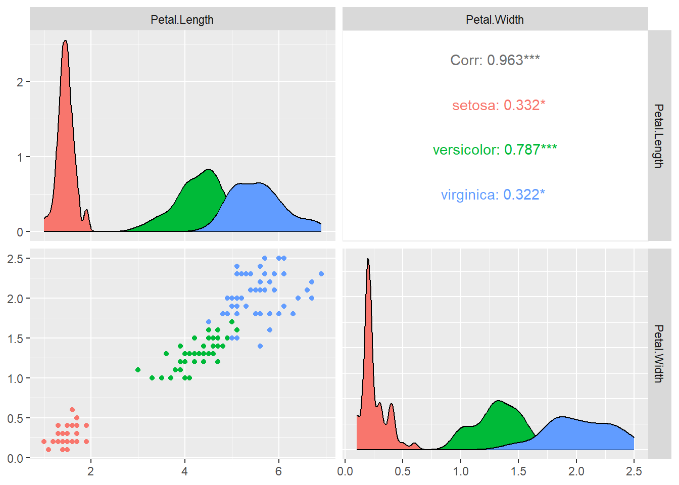
We can see from the plots that relationship between petal width and petal length differs by the species. Let us for now focus only on the versicolor species.
Let us first subset the dataset by versicolor, which contains information about the versicolor species only.
versicolor <- subset(iris, Species == "versicolor" )

head(versicolor, 5)
## Sepal.Length Sepal.Width Petal.Length Petal.Width Species
## 51 7.0 3.2 4.7 1.4 versicolor
## 52 6.4 3.2 4.5 1.5 versicolor
## 53 6.9 3.1 4.9 1.5 versicolor
## 54 5.5 2.3 4.0 1.3 versicolor
## 55 6.5 2.8 4.6 1.5 versicolorLet’s plot the petal width vs petal length
ggplot(versicolor, aes(x = Petal.Length, y = Petal.Width)) + geom_point()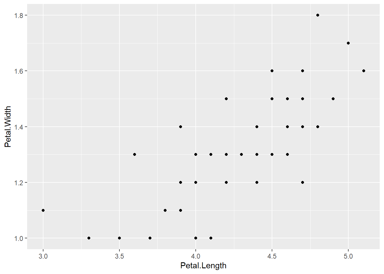
We can see that there is a strong pattern in the data. The relationship looks quite strong and linear.
Fitting a linear regression model with lm()
Let us use petal width as response variable and petal length as an explanatory variable. We will fit model of the form \[\hat{y} = \beta_0 + \beta_1 x\]
mod1 <- lm(Petal.Width ~ Petal.Length, data=versicolor)lm() function comes with few utility functions like
coef()to generate model coefficients.fitted()to generate the fitted values.residuals()to generate the residuals.summary()to produce model summaries.plot()to produce diagnostic plots.predict()to make predictions using the model.
For example the model coefficients are
coef(mod1)## (Intercept) Petal.Length
## -0.08428835 0.33105360i.e
- intercept = -0.084
- slope = 0.33
We can add the fitted model to the graph including the standard error
ggplot(versicolor, aes(x = Petal.Length, y = Petal.Width)) + geom_point() + geom_smooth(method = "lm", se = TRUE)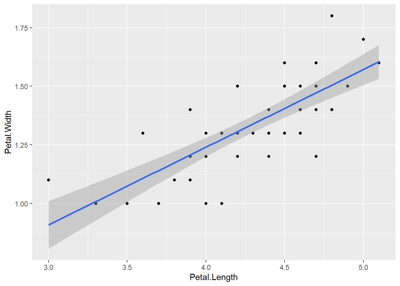
Overview with summary() function
The function summary() gives the summary of the linear model we have fitted
summary(mod1)##
## Call:
## lm(formula = Petal.Width ~ Petal.Length, data = versicolor)
##
## Residuals:
## Min 1Q Median 3Q Max
## -0.273031 -0.073373 -0.006479 0.086271 0.295231
##
## Coefficients:
## Estimate Std. Error t value Pr(>|t|)
## (Intercept) -0.08429 0.16070 -0.525 0.602
## Petal.Length 0.33105 0.03750 8.828 1.27e-11 ***
## ---
## Signif. codes: 0 '***' 0.001 '**' 0.01 '*' 0.05 '.' 0.1 ' ' 1
##
## Residual standard error: 0.1234 on 48 degrees of freedom
## Multiple R-squared: 0.6188, Adjusted R-squared: 0.6109
## F-statistic: 77.93 on 1 and 48 DF, p-value: 1.272e-11This gives
- summary of residuals
- The coefficient estimates and their standard errors
- P-values for individual estimates as well as F-statistics for the significance of the overall model.
- \(R^2\) values, % of variation explained by the model.
F-statistic: 77.93 on 1 and 48 DF, p-value: 1.272e-11 is significant, so Petal.Length is useful in predicting Petal width.
\(R^2 = 0.618\) means that 61.8% of the variation in Petal width is explained by this model using petal length.
Model equation
The predicted model equation is
\[\widehat{Petal.Width} = -0.084 + 0.33 \times Petal.Length\] ### Interpretation of coefficients
- \(\beta_0 = -0.084\), the average petal width is -0.084, when both the petal length is 0. Usually intercept is not very informative as in case here.
- \(\beta_1 = 0.33\), for every unit increase in petal length, petal width will increase by 0.254 on average.
Diagnostics plot with plot() function
par(mfrow = c(2,2))

plot(mod1)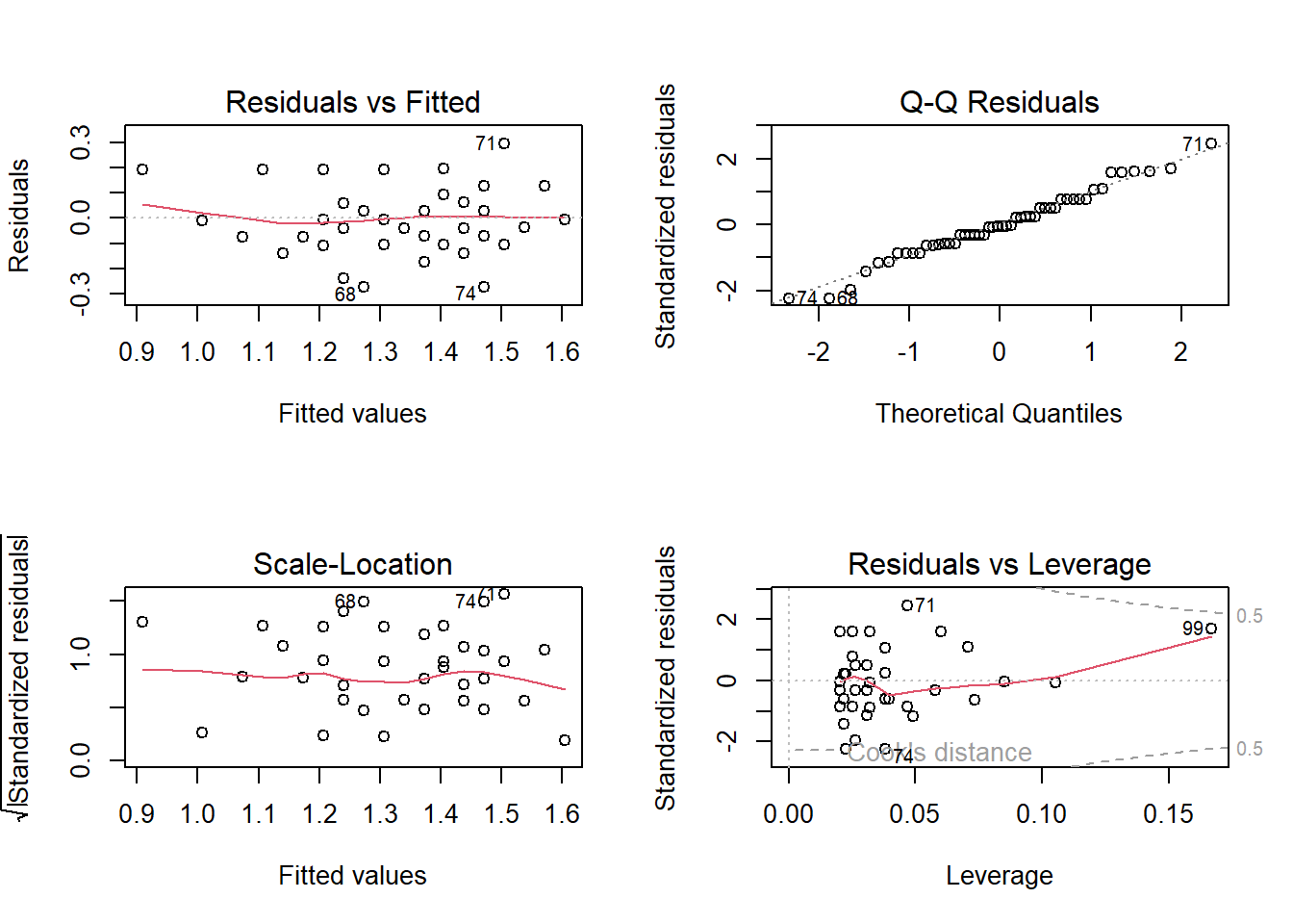
Residual vs Fitted plot : Check if the residual exhibits a clear pattern and if the residuals are randomly scattered around 0.
Q-Q Residuals plot : Check if the residual follows a linear trend with no obvious shape or deviation.
Scale-Location: Same as first plot but plotted on different scale.
Residual vs Leverage: Check for obvious groups and if points are too far from the center.
Prediction with predict() fucntion
Using the fitted model, let us predict the Petal.Width of versicolor species with Petal.Length=4.8,
petal_new <- data.frame(Petal.Length= 4.8) # Define a new data.frame with Petal;length = 4.8
mod1.pred = predict(mod1, newdata = petal_new )
mod1.pred
## 1
## 1.504769More predictors
When we have two continous predictors, we will fit model of the form
\[\hat{y} = \beta_0 + \beta_1 x_1 + \beta_2 x_2 +.....\]
Let us include additional additional variable Sepal.Width in order to estimate the Petal.Width,
mod2 <- lm(Petal.Width ~ Petal.Length +Sepal.Width, data=versicolor)
summary(mod2)
##
## Call:
## lm(formula = Petal.Width ~ Petal.Length + Sepal.Width, data = versicolor)
##
## Residuals:
## Min 1Q Median 3Q Max
## -0.270959 -0.064119 -0.005774 0.072671 0.248525
##
## Coefficients:
## Estimate Std. Error t value Pr(>|t|)
## (Intercept) -0.32521 0.16312 -1.994 0.05201 .
## Petal.Length 0.25433 0.04118 6.177 1.45e-07 ***
## Sepal.Width 0.20496 0.06166 3.324 0.00173 **
## ---
## Signif. codes: 0 '***' 0.001 '**' 0.01 '*' 0.05 '.' 0.1 ' ' 1
##
## Residual standard error: 0.1122 on 47 degrees of freedom
## Multiple R-squared: 0.6914, Adjusted R-squared: 0.6783
## F-statistic: 52.65 on 2 and 47 DF, p-value: 1.002e-12F-statistic: 52.65 on 2 and 47 DF, p-value: 1.002e-12 is significant, so at least one predictors is useful in predicting petal width. We can see that both the predictor are also statistically significant.
\(R^2 = 0.67\) means that 67% of the variation in petal width is explained by this model using petal length and sepal width.
Model Equation
The predicted model equation is
\[\widehat{Petal.Width} = -0.325 + 0.254 \times Petal.Length+ 0.205 \times Sepal.Width \]
Interpretation of coefficients
- \(\beta_0 = -0.325\), the average petal width is -0.325, when both the petal length and sepal width are 0. Usually intercept is not very informative as in case here.
- \(\beta_1 = 0.254\), for every unit increase in petal length, petal width will increase by 0.254 on average, holding sepal width constant.
- \(\beta_2 = 0.205\), for every unit increase in sepal width, petal width will increase by 0.205 on average, holding petal length constant.
Diagnostic plots
par(mfrow = c(2,2))

plot(mod2)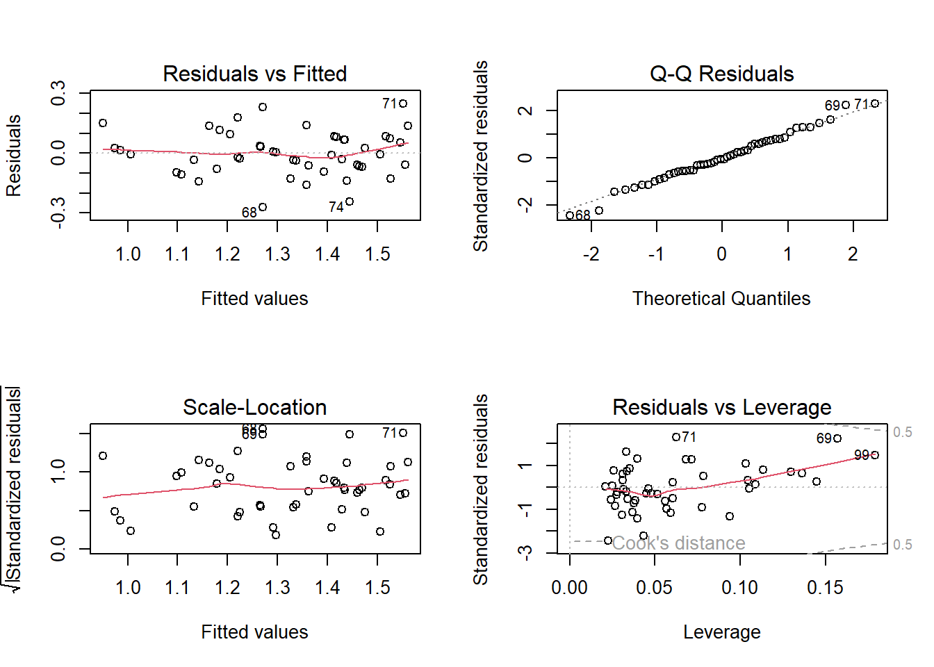
Multicollinearity
When fitting multiple linear regression, we need to be careful of
Multicollinearity. Multicollinearity is the occurrence high correlation
with the two or more predictor variables in a multiple regression model.
Each regression coefficient is interpreted as mean change in the
response bariable assuming other variables are held constant. But if two
or more predictor variables are highly correlated, it is difficult to
change one variable without changing another. One way to detect using
the variance inflation factor (VIF), which measures
strength of correlation between the predictor variables in a regression
model. We can us use the vif() function from the car
library to calculate the VIF for each predictor variable in the model.
Generally VIF of less than 5 is not an issue.
library(car)## Warning: package 'car' was built under R version 4.3.2## Warning: package 'carData' was built under R version 4.3.2vif(mod2)## Petal.Length Sepal.Width
## 1.458119 1.458119Categorical predictors
Analysis of variance is the modeling technique used when the response variable is continuous and the explanatory variable is categorical. When there is only two levels, this is basically the t.test.
An anova in R is executed with the aov( ) function. From
the iris data, let look at the difference in petal
length between the three species. Lets visualize the relationship
between petal length and species using a boxplot.
Assumptions of ANOVA
- Independence of observations: Checked by considering the study design.
- Normality of response variable for each population: Refer to the boxplot.
- Must have same population standard deviation. Rule of thump, we can check if the ratio of largest standard deviation and smallest standard deviation among group is less than 2.
ggplot(iris, mapping=aes(x=Species, y=Petal.Length, fill = Species))+geom_boxplot()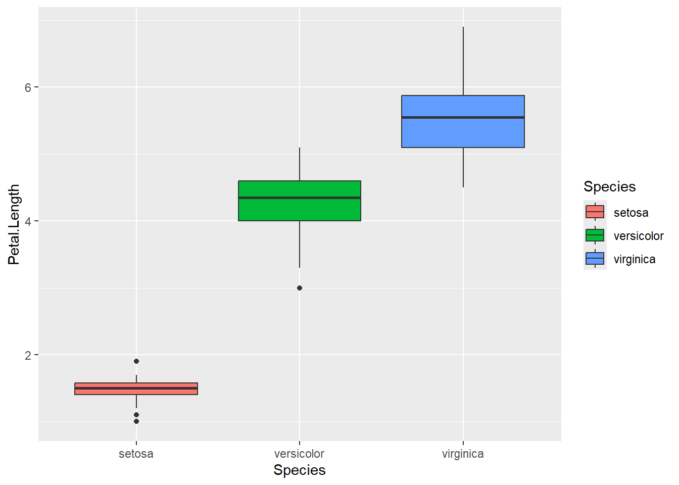
Calculate the standard deviations
tapply(iris$Petal.Length,iris$Species, sd)## setosa versicolor virginica
## 0.1736640 0.4699110 0.5518947Fit the ANOVA model
mod3 <- aov(Petal.Length~Species, data=iris)
summary(mod3)
## Df Sum Sq Mean Sq F value Pr(>F)
## Species 2 437.1 218.55 1180 <2e-16 ***
## Residuals 147 27.2 0.19
## ---
## Signif. codes: 0 '***' 0.001 '**' 0.01 '*' 0.05 '.' 0.1 ' ' 1We can see the F-statistic and the p-value associated with that. P-value is significant, so we can say that there is difference in petal length among the species.
To specify the difference between each groups, we can use a pairwise
test using the pairwise.t.test() in \(R\). We will specify that
p.adj=‘bonf’ as we need to adjust the p-values for
doing multiple comparisons.
pairwise.t.test(iris$Petal.Length, iris$Species, p.adj='bonf')##
## Pairwise comparisons using t tests with pooled SD
##
## data: iris$Petal.Length and iris$Species
##
## setosa versicolor
## versicolor <2e-16 -
## virginica <2e-16 <2e-16
##
## P value adjustment method: bonferroniThere are 3 groups, so we have 3 pairwise comparisons to look at. We can see that all the 3 p-values are significant.
Fitting lm() for categorical predictor
For a categorical predictor with levels A, B, C…., we can also fit a similar linear model of the form \[\hat{y} = \beta_0 + \beta_1 x_1 + \beta_2 x_2.......\] Where
- Base/reference level is level A
- \(x_1 =1\) if it is in level B, and 0 otherwise
- \(x_2 =1\) if it is in level C, and 0 otherwise…and so on
The intercept \(\beta_0\) is the mean for the base level. \(\beta_1\) is the mean difference between level B and level A. \(\beta_2\) is the mean difference between level C and level A.
Lets fit the linear model for the above question
mod4 <- lm(Petal.Length~Species, data=iris)
summary(mod4)
##
## Call:
## lm(formula = Petal.Length ~ Species, data = iris)
##
## Residuals:
## Min 1Q Median 3Q Max
## -1.260 -0.258 0.038 0.240 1.348
##
## Coefficients:
## Estimate Std. Error t value Pr(>|t|)
## (Intercept) 1.46200 0.06086 24.02 <2e-16 ***
## Speciesversicolor 2.79800 0.08607 32.51 <2e-16 ***
## Speciesvirginica 4.09000 0.08607 47.52 <2e-16 ***
## ---
## Signif. codes: 0 '***' 0.001 '**' 0.01 '*' 0.05 '.' 0.1 ' ' 1
##
## Residual standard error: 0.4303 on 147 degrees of freedom
## Multiple R-squared: 0.9414, Adjusted R-squared: 0.9406
## F-statistic: 1180 on 2 and 147 DF, p-value: < 2.2e-16We can see that the overall F-statistic: 1180 on 2 and 147 DF, p-value: < 2.2e-16 is same as above.
Here the base/reference level is setosa. If you don’t specify, \(R\) will level them alphabetically.
Model equation
The predicted model equation is
\[\widehat{Petal.Length} = 1.46 + 2.80 \times Species_{Versicolor} + 4.09 \times Species_{Virginica}\]
Interpreatation of coefficients
- \(\beta_0 = 1.46\), mean petal length for setosa species is 1.46.
- \(\beta_1 = 2.80\), difference in mean petal length between Versicolor and setosa species is 2.80.
- \(\beta_2 = 4.09\), difference in mean petal length between Virginica and setosa species is 4.09.
Diagnostic plots
par(mfrow = c(2,2))

plot(mod4)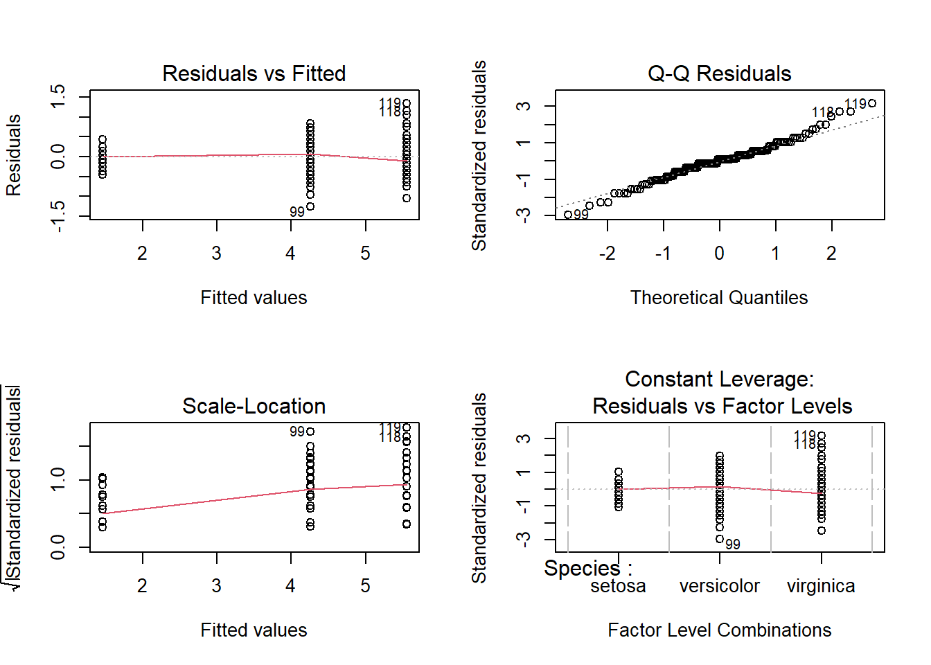
Linear model with interaction
The multiple regression model assumes that when one of the predictors is changed by 1 unit and the values of the other variables remain constant, the predicted response changes by \(\beta_j\).
A statistical interaction occurs when this assumption is not true, such that the effect of one explanatory variable on the response depends on other explanatory variables.
Here we specifically examine interaction in a two-variable setting, where one of the predictors is categorical and the other is numerical.
For example, the effect of petal width on petal length may be dependent on the species of the flowers. This dependency is known as an interaction effect.
Plotting interactions
We can use interaction_plot() function from
interactions package, as follows
library(interactions)## Warning: package 'interactions' was built under R version 4.3.3mod5<- lm(Petal.Length ~ Petal.Width * Species, data = iris)
interact_plot(mod5, pred = Petal.Width, modx = Species,
plot.points = TRUE)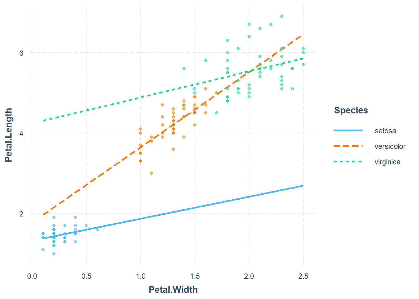
Here we will fit model of the form
\[\hat{y} = \beta_0 + \beta_1 x_1 + \beta_2 x_2+ \beta_3 x_3 + \beta_4 x_1 \times x_2 + \beta_5 x_1 \times x_3 \] where
- Base/reference level is species setosa
- \(x_1\) is Petal.Width
- \(x_2 =1\) if it is in species Versicolor, and 0 otherwise
- \(x_3 =1\) if it is in species Virginica , and 0 otherwise
mod5<- lm(Petal.Length ~ Petal.Width * Species, data = iris)
anova(mod5)
## Analysis of Variance Table
##
## Response: Petal.Length
## Df Sum Sq Mean Sq F value Pr(>F)
## Petal.Width 1 430.48 430.48 3294.5561 < 2.2e-16 ***
## Species 2 13.01 6.51 49.7891 < 2.2e-16 ***
## Petal.Width:Species 2 2.02 1.01 7.7213 0.0006525 ***
## Residuals 144 18.82 0.13
## ---
## Signif. codes: 0 '***' 0.001 '**' 0.01 '*' 0.05 '.' 0.1 ' ' 1summary(mod5)##
## Call:
## lm(formula = Petal.Length ~ Petal.Width * Species, data = iris)
##
## Residuals:
## Min 1Q Median 3Q Max
## -0.84099 -0.19343 -0.03686 0.16314 1.17065
##
## Coefficients:
## Estimate Std. Error t value Pr(>|t|)
## (Intercept) 1.3276 0.1309 10.139 < 2e-16 ***
## Petal.Width 0.5465 0.4900 1.115 0.2666
## Speciesversicolor 0.4537 0.3737 1.214 0.2267
## Speciesvirginica 2.9131 0.4060 7.175 3.53e-11 ***
## Petal.Width:Speciesversicolor 1.3228 0.5552 2.382 0.0185 *
## Petal.Width:Speciesvirginica 0.1008 0.5248 0.192 0.8480
## ---
## Signif. codes: 0 '***' 0.001 '**' 0.01 '*' 0.05 '.' 0.1 ' ' 1
##
## Residual standard error: 0.3615 on 144 degrees of freedom
## Multiple R-squared: 0.9595, Adjusted R-squared: 0.9581
## F-statistic: 681.9 on 5 and 144 DF, p-value: < 2.2e-16We can see that the overall model is F-statistic: 562.9 on 5 and 144 DF, p-value: < 2.2e-16, which is significant. From the ANOVA table, the interaction and main effect terms are all significant.
Model equation
The predicted model equation is
\[\widehat{Petal.Length} = 1.328 + 0.547 \times Petal.Width + 0.454 \times Species_{Versicolor} + 2.913 \times Species_{Virginica} + 1.323 \times Petal.Width \times Species_{Versicolor} + 0.101 \times Petal.Width \times Species_{Virginica} \]
Interpretation of coefficients
- \(\beta_0 = 1.328\), is average petal length for setosa species when petal width is 0.
- \(\beta_1 = 0.547\), for every unit
increase in petal width, petal length will increase by 0.065 on
average.
- \(\beta_2 = 0.453\), average difference in petal length between versicolor and setosa species is 0.4533, holding petal width constant.
- \(\beta_3 = 2.913\), average difference in petal length between virginica and setosa species is 2.913, holding petal width constant.
- \(\beta_4 = 1.323\), for every unit increase in petal width, average difference in petal length between versicolor and setosa species will be increased by 1.323.
- \(\beta_5 = 0.101\), for every unit increase in petal width, difference in mean petal length between virginica and setosa species will be increased by 0.101.
Diagnostic plots
par(mfrow = c(2,2))

plot(mod5)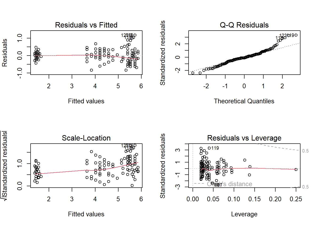
Prediction with predict() fucntion
Using the fitted model, let us predict the Petal.Width of versicolor species with Sepal.Width = 2.9.
petal_new <- data.frame(Petal.Width = 1.4, Species = "versicolor")
mod5.pred = predict(mod5, newdata = petal_new )
mod5.pred
## 1
## 4.39833Logistic regression
A logistic regression is used when there is one binary response variable (yes/no, success/failure) and continuous, categorical or multiple predictor variables which is related to the probability or odds of the response variable.
If \(p\) is the probability of an outcome occurring then,
\[\mbox{ odds } = \frac{p}{1-p} \]
- The range of probability is 0 to 1.
- The range of odds is 0 to + \(\infty\).
- If we take log of odds, then the range is from \(- \infty\) to \(+ \infty\).
So, suppose \(Y\) is a binary response variable and \(x_1, x_2, x_3....\) are a predictor variable, we fit model of the form
\[ ln(\frac{\hat{p}}{1-\hat{p}}) = \beta_0 + \beta_1 x_1+ \beta_2 x_2.....\] Where \(\hat{p}\) is the expected proportion of success.
Fitting a logistic regression model using glm()
We can use glm() function to fit a logistic regression
model. As in the lm(), the important argument is the model
formula. We also need to specify that
family="binomial".
We will demonstrate the usage of logistic regression using the R built-in data called mtcars. You can read more about the dataset using
?mtcarsdata(mtcars)
head(mtcars)## mpg cyl disp hp drat wt qsec vs am gear carb
## Mazda RX4 21.0 6 160 110 3.90 2.620 16.46 0 1 4 4
## Mazda RX4 Wag 21.0 6 160 110 3.90 2.875 17.02 0 1 4 4
## Datsun 710 22.8 4 108 93 3.85 2.320 18.61 1 1 4 1
## Hornet 4 Drive 21.4 6 258 110 3.08 3.215 19.44 1 0 3 1
## Hornet Sportabout 18.7 8 360 175 3.15 3.440 17.02 0 0 3 2
## Valiant 18.1 6 225 105 2.76 3.460 20.22 1 0 3 1As vsEngine (0 = V-shaped, 1 = straight) is a binary
variable, we will use it as response variable, mpg
Miles/(US) gallon as a continuous predictor variable.
table(mtcars$vs)##
## 0 1
## 18 14mod6 <- glm(vs ~ mpg , data=mtcars, family=binomial)
summary(mod6)##
## Call:
## glm(formula = vs ~ mpg, family = binomial, data = mtcars)
##
## Coefficients:
## Estimate Std. Error z value Pr(>|z|)
## (Intercept) -8.8331 3.1623 -2.793 0.00522 **
## mpg 0.4304 0.1584 2.717 0.00659 **
## ---
## Signif. codes: 0 '***' 0.001 '**' 0.01 '*' 0.05 '.' 0.1 ' ' 1
##
## (Dispersion parameter for binomial family taken to be 1)
##
## Null deviance: 43.860 on 31 degrees of freedom
## Residual deviance: 25.533 on 30 degrees of freedom
## AIC: 29.533
##
## Number of Fisher Scoring iterations: 6Goodness of fit of the glm()
Deviance is the measure of goodness of fit of the glm. The residual deviance has an approximate \(\chi^2\) distribution. we can test the goodness of fit by
pchisq(df=30,q=25.533,lower.tail=F)## [1] 0.6987382This is not significant, hence the model provides an adequate fit to the data.
Model equation
The predicted model equation is
\[ ln(\frac{\hat{p}}{1-\hat{p}}) = -8.833 + 0.430 \times mpg\]
Interpretation of coefficeints
- \(\beta_0 = -8.833\), when mpg is
0, the log odds of
vs =1is -8.833. i.e, the odds of havingvs =1is \(e^{-8.833} = 0.00014\), when mpg = 0. - \(\beta_1 = 0.430\), for every one
unit increase in mpg, the estimated log odds of having
vs =1is increased by 0.430. i.e, for every increase in mpg, odd of `vs =1’ is increase by \(e^{0.430} = 1.537\) .