Core Statistical Programming
This section introduces some of the core concepts and control structures needed to write programs in R. You should always write your code in a script, this is particularly important when you are writing programs that cover multiple lines, as a script allows the user to organise and execute large portions of code in one go. The logical flow of a script is controlled using control structures such as loops and if statements.
Logical operators
R has the following logical operators which can be used to compare objects and perform calculations with logical values
==Equals!=Not equal>=Greater than or equal>Greater than<=Less than or equal<Less than||or&&and!xnot x
The first 6 of these allow us to compare objects in R. Each of these
operators returns either TRUE or FALSE.
x <- 'a character string'
y <- 'a different string'

x == y #Check if x equals y
## [1] FALSEThe two strings in the example are different so R has returned the
logical value FALSE.
x != y #Check if x is different from y## [1] TRUEThe operators || , && ,
! deal exclusively with logical values and allow us to
perform calculations with logical values. Let P and Q denote two logical
variables. The operator || can be read as ‘or’. For
instance P||Q is read as ‘P or Q’ and returns
TRUE if either P or Q equals TRUE. Likewise,
P&&Q is read as ‘P and Q’ and returns
TRUE only if both P and Q equal TRUE. Finally
! negates a logical value and is read as ‘not’. We can
record the result of the operators with a simple truth table
| P | Q | !P | P || Q | P && Q |
| TRUE | TRUE | FALSE | TRUE | TRUE |
| TRUE | FALSE | FALSE | TRUE | FALSE |
| FALSE | TRUE | TRUE | TRUE | FALSE |
| FALSE | FALSE | TRUE | FALSE | FALSE |
It is useful to remember that == (which is used to
compare values), is different to = (which is used for
assignment and function arguments). It is easy to make typos between the
two.
If Statements
If statements are an extremely useful control structure in any programming language. An if statement allows you execute a portion of code provided a given condition holds. The general structure of an if statement is as follows
if(condition){
  #do something
}
The condition that we would like to test is written in the parentheses, and the code to be executed is written between the curly brackets. For example,
x <- 5

if(x >= 4){

  x <- x-1

}

print(x)
## [1] 4We first check the logical condition x >= 4, this can
either take the value TRUE or FALSE, since the
value in this case is TRUE, the code in the curly braces is
executed and the value of x is updated. To add additional
conditions to an if statement we use the else if phrase,
x <- 1

if(x >= 4){

  x <- x-1

  }else if(x <= 2){ #In this case the second condition is satisfied and not the first

    x <- x+1

}

print(x)
## [1] 2We can add as many conditions as we like to an if statement using the
else if phrase. It can be helpful to visualize the logical
flow of the code with a flowchart
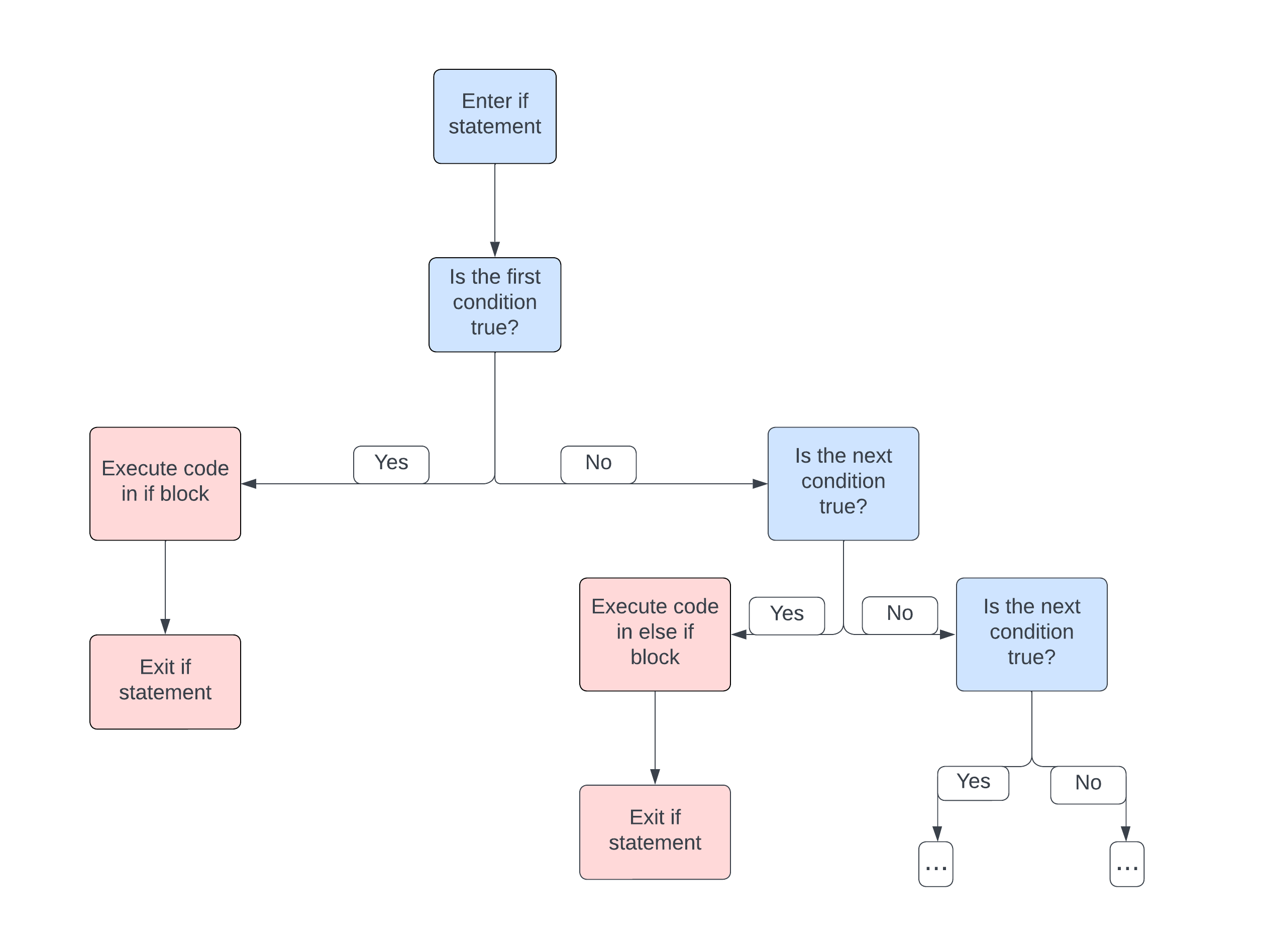
At the end of an if statement you can add an else section, this section is executed in the case when none of the conditions above it are satisfied.
x <- 3

if(x >= 4){

  x <- x-1

  }else if(x <= 2){

    x <- x+1

  }else{ # x equals 1 so the two previous conditions are not satisfied

  x <- 2*x

}
print(x)
## [1] 6Using the logical operators we can create more complicated conditions within an if statement.
x <- 6

if(x >= 4 && x != 6){ #String together multiple logical conditions

  x <- x-1

  }else if(x <= 2){

    x <- x+1

  }else{

  x <- 2*x

}

print(x)
## [1] 12If you wish to test many possible conditions, you can consider the
case_when() function in the dplyr library,
rather than nesting many if statements.
For Loops
For loops allow the user to run a portion of code repeatedly for a specified number of iterations. Usually we define a vector of elements which we wish to iterate over, for each element in the vector we assign its value to the iterating variable.
for(i in 1:10){ #i is the iterating variable

  print(i^2)

  }
## [1] 1
## [1] 4
## [1] 9
## [1] 16
## [1] 25
## [1] 36
## [1] 49
## [1] 64
## [1] 81
## [1] 100More often than not, a for loop iterates over a sequence of integers, as in the example above, however this need not always be the case. In fact, any vector or list can be iterated over in a for loop.
vec <- c(TRUE,FALSE,TRUE,TRUE)

for(i in vec){

  print(i)

}
## [1] TRUE
## [1] FALSE
## [1] TRUE
## [1] TRUEIt is also possible to define for loops within another for loop, this structure is called a nested for loop and can be useful when performing calculations on the elements of an array or data frame.
m <- matrix(nrow = 6, ncol = 6)

for(i in 1:6){ #index over rows

    for(j in 1:6){ #index over columns

      m[i,j] = i+j

    }
}

print(m)
## [,1] [,2] [,3] [,4] [,5] [,6]
## [1,] 2 3 4 5 6 7
## [2,] 3 4 5 6 7 8
## [3,] 4 5 6 7 8 9
## [4,] 5 6 7 8 9 10
## [5,] 6 7 8 9 10 11
## [6,] 7 8 9 10 11 12While Loops
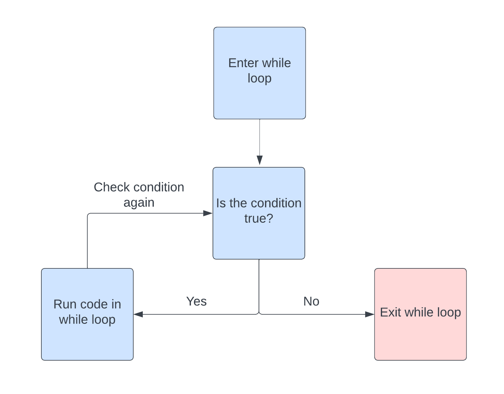
Like the for loop, a while loop is another control structure which allows us to repeat a portion of code. However, instead of iterating over the elements of a vector, a while loop iterates while a condition is true. The general structure of a while loop is as follows.
while(condition){
  #do something
}
This can be visualized nicely in a flow chart
For example,
x <- 1

while(x <= 10){

  print(x^2)

  x <- x+1
}
## [1] 1
## [1] 4
## [1] 9
## [1] 16
## [1] 25
## [1] 36
## [1] 49
## [1] 64
## [1] 81
## [1] 100Unlike the for loop, there is a possibility that a while loop will run infinitely (or until your computer runs out of memory). This happens when the condition is always satisfied, for example
x <- 1

while(x>0){

  x <- x+1 #x will always be positive

}
It may not always be easy to tell whether a while loop will terminate or not before running it, this means one should exercise caution when using while loops, especially for time intensive calculations. How can we decide weather the following while loop will terminate without running it? See https://en.wikipedia.org/wiki/Collatz_conjecture.
x <- 5231521

while(x != 1){

    if(x%%2 == 0){

      x <- x/2

    }else{

      x <- 3*x+1

    }
}
%% is called the modulus operator and gives the
remainder after division, see https://en.wikipedia.org/wiki/Modulo.
R has two additional control structures associated to loops, these
are next and break. The next
keyword can be used to skip an iteration in a loop and the
break keyword can be used to exit a loop entirely.
Generally these are used in conjunction with an if statement, for
example
for(i in vector){ #works with for loops and while loops

  if(condition){
    next
  }

}
And
for(i in vector){  #works with for loops and while loops

  if(condition){
    break
  }

}
apply(), lapply()
Apply functions provide a useful and concise way to apply a function to chunks of data, for instance the rows or columns of a matrix or the elements of a list. The apply functions can often be used in place of loops and can make your code more readable.
The function apply() applies a function to the margins
of an array or matrix and returns the result as a vector, array or list
depending on the function being applied. apply() takes
arguments apply(X, MARGIN, FUN, ...). Here X
is a matrix or array, MARGIN is a vector which specifies
the subscripts which the function will be applied to and
FUN is a function. For example, when X is a
matrix, MARGIN = 1 indicates the first index, i.e. the rows
of the matrix. Likewise, MARGIN = 2 means that the function
will be applied to the columns of the matrix.
m <- matrix(data = runif(20,0,1) ,nrow = 4 , ncol = 5)

apply(m, 1, mean)
## [1] 0.5454088 0.4298622 0.6577721 0.4443690lapply() applies a function to the elements of a vector
or list. Unlike apply(), lapply() always
returns a list. The arguments of lapply() are
lapply(X, FUN, ...), where X is a vector or
list and FUN is a function.
my_list <- list(c(0,pi/2,pi), c(1,2,3))

lapply(my_list,sin)
## [[1]]
## [1] 0.000000e+00 1.000000e+00 1.224606e-16
##
## [[2]]
## [1] 0.8414710 0.9092974 0.1411200Another apply function is sapply(),
sapply() is essentially the same as lapply()
however sapply() attempts to simplify the result by
returning a vector or array instead of a list.
Vectorisation
Loops are an essential part of programming in any language, however
they can significantly increase the run time of a program, especially
when there are many nested loops. The idea behind vectorisation is to
replace loops, wherever possible, with operations applied to a whole
vector of values simultaneously. Here is a simple example, the vectors
x and y can be added using a for loop
x <- 1:10

y <- 10:1

z <- vector(length = 10)

for(i in 1:length(z)){

  z[i] <- x[i] + y[i]

}
print(z)
## [1] 11 11 11 11 11 11 11 11 11 11However, this operation can be vectorised in R simply by using the
addition operator +.
x <- 1:10

y <- 10:1

z <- x + y

print(z)
## [1] 11 11 11 11 11 11 11 11 11 11The difference is subtle, because both of these examples produce the same output, but the later is much more efficient. In general, if you can replace a loop with a vectorised expression without any significant loss to code readability, it is usually beneficial to do so. Most functions that are built in to R are vectorised.
User Defined Functions
R allows users to create and use their own functions. To define a function in R we use the following syntax
my_function <- function(argument1, argument2, etc...){

  #Do something

}
Using a user defined function works in exactly the same way as any other function in R, simply by calling the function name with the appropriate inputs in parentheses. As a simple example, we can write a function to calculate the mean of a numeric vector.
vec <- 1:10

my_mean <- function(x){

  sum(x)/length(x)

}

my_mean(vec)
## [1] 5.5Within the function my_mean() we have used
sum() and length(). When defining a function
you can call any other functions within that function. Moreover, you can
also define other functions within a function, often this can lead to
more organised and understandable code. Suppose we don’t have the
sum() function at our disposal. We could define our own sum
function within the function my_mean().
vec <- 1:10

my_mean <- function(x){

  my_sum <- function(y){ #Define a function to sum a vector

    s <- 0

    for(i in 1:length(y)){

      s <- s + y[i]

    }

   return(s)

  }

  return(my_sum(x)/length(x))

}

my_mean(vec)
## [1] 5.5return() allows us to specify the value which the
function returns, or ‘’outputs’’. If return is not called then the
function will automatically return the value of the last evaluated
expression.
It is important to note that my_sum() only exists
locally within my_mean(). That is, my_sum()
cannot be used outside of the function my_mean(). In
general, any assignment made within a function exists only locally.
Example: The Central Limit Theorem
One of the fundamental results in probability is the central limit theorem. The statement of the central limit theorem is as follows.
Let \(\xi_1,\dots, \xi_n\) be independently and identically distributed random variables with \(\mathbb{E}[\xi_i] = \mu\) and \(\text{Var}[\xi_i] = \sigma^2\) for each \(i\). Then the distribution of the random variable
\[ \tau_n = \frac{\sum_{i=1}^{n}\xi_i - n\mu}{\sqrt{n}\sigma} \]
converges to the standard normal distribution as n tends to \(\infty\).
In this example we will use R to run some computational experiments and investigate the central limit theorem for a given initial distribution.
Define a random variable,
\[ \tau = \frac{\sum_{i=1}^n \xi_i -n\mu}{\sqrt{n}\sigma} \]
as a function of \(n\) random
numbers \(\xi_1 , \dots , \xi_n\) where
each \(\xi_i\) is uniformly distributed
on the interval \((0,1)\). We will
explore the distribution of \(\tau\) as
\(n\) increases. For this we will use
some features from the tidyverse package.
Firstly, let us create a function to evaluate \(\tau\), to do this we first need to calculate the mean and variance of each \(\xi_i\).
The mean is given by the formula,
\[ \mathbb{E}[\xi_i] = \int_0^1 x dx = \frac{1}{2} \]
and the variance is calculated by the formula
\[ \begin{align*} Var[\xi_i] &= \mathbb{E}[\xi_i^2]-\mathbb{E}[\xi_i]^2 \\ &= \int_0^1 x^2dx - \frac{1}{4}\\ &= \frac{1}{12} \end{align*} \]
The tau function can now be implemented in R
tau <- function(x){

  return((1/(sqrt(length(x))*sqrt(1/12)))*(sum(x)-length(x)*0.5))

}
Now we can generate samples of \(\tau\) for different values of \(n\) using the following script
#Define a vector of different values of n which will be tested
N <- c(1,10,100,1000)

#Define the number of samples
nsamps <- 10000

#Create a generic data frame
df <- tibble(.rows = nsamps)

for(n in 1:4){

  tau_vec <- vector(mode = 'numeric', length = N[n]) #create a generic vector

    for(i in 1:nsamps){

      #Generate a vector of uniformly distributed random numbers
      xi <- runif(N[n], 0, 1)

      #Apply the tau function
      tau_vec[i] <- tau(xi)

    }
  #Add data to data frame
  df[n] <- tau_vec
}
The following plot compares the distribution of the samples for the different values of \(n\).
#plotting code

#Define names for the columns of the data frame
names(df) <- c('n = 1','n = 10','n = 100','n = 1000')

#plots

plot1 <- ggplot(df, aes(x=`n = 1`))+geom_histogram(aes(y = after_stat(density)),binwidth = 0.1)

plot2 <- ggplot(df, aes(x=`n = 10`))+geom_histogram(aes(y = after_stat(density)),binwidth = 0.1)

plot3 <- ggplot(df, aes(x=`n = 100`))+geom_histogram(aes(y = after_stat(density)),binwidth = 0.1)

plot4 <- ggplot(df, aes(x=`n = 1000`))+geom_histogram(aes(y = after_stat(density)),binwidth = 0.1)


grid.arrange(plot1, plot2, plot3, plot4, ncol=2) #this comes from the gridExtra package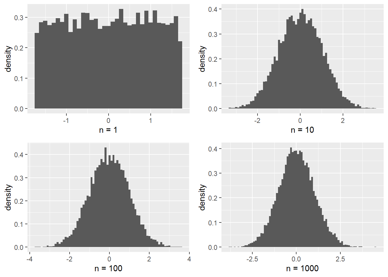
Comparing the empirical CDF obtained for \(n=1000\) with the CDF of the standard normal distribution yields the plot
# Create a sequence of values for x-axis
x_values <- seq(-3, 3, length.out = 10000)

# Calculate the CDF values for the standard normal distribution
cdf_values <- pnorm(x_values)

# Combine x, CDF values and emperical data into a data frame
data <- tibble(x = x_values, cdf = cdf_values, emp_dat = tau_vec)

#Create plot
ggplot(data) +
  geom_line(aes(x = x, y = cdf, colour = "Standard Normal"), linewidth = 1) +
  stat_ecdf(aes(x = emp_dat, colour = "n = 1000 empirical CDF"), geom = "step") +
  labs(x = "x", y = "CDF") +
  scale_color_manual(values = c("red", "blue"),
labels = c("Standard Normal", "n = 1000 empirical CDF")) 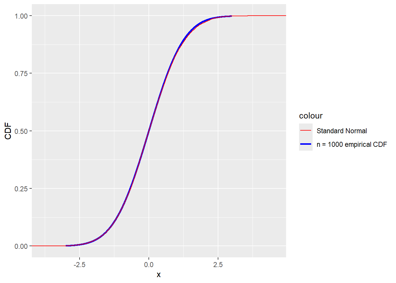
Indeed the distribution of \(\tau\) appears to be approaching the standard normal distribution for large \(n\).