Variables and types of R objects
This section introduces some fundamental concepts that will help you understand how to use R.
R as a calculator
R can be used both as an interactive environment and as a language for programming. You should almost always type your R commands in a script (so you have a record of what you have done), and then as you run them (either by pressing the run button or using a shortcut) they are sent to the console and evaluated. The simplest commands involve using R to do simple mathematical calculations, like:
2*3 #Multiplication ## [1] 628/5 #Division## [1] 5.63+6 #Addition ## [1] 94-9 #Subtraction## [1] -5Many familiar mathematical functions are also available to us,
sin(pi) #Note that the answer may not be exactly zero due to computational errors## [1] 1.224606e-16cos(0) #note also that trig functions like sin() and cos() operate in radians by default## [1] 1log(1) #The natural logarithm## [1] 0exp(3) #The exponential e^x## [1] 20.08554Variables
A variable is a piece of memory allocated for the storage of
specific data. In R, a variable is created by assigning a name to an
object, this can be done using the assignment operator
<-. That is a less than sign followed by a minus sign.
For example,
x <- 2 # An integer
y <- "Hello World" #A character String
z <- TRUE #A Logical Value
The name given to an object can be almost anything provided the first
character is not a number or one of the special characters:
^, ! , $ , @ ,
+ , - , / , *.
Once a variable has been created, it can be interacted with and used in calculations simply by using its name.
x^2 ## [1] 4Some terminology
Everything that we interact with in R is called an object. For example, numbers, vectors, lists and data frames are all objects. Each object belongs to a specific class. R has five atomic classes or data types. All other data types are constructed from these basic data types. These are
Character
Numeric (real numbers/floating point)
Integer
Complex (complex number)
Logical
To check the class of an object, we use the function
class() applied to the object.
a_number <- 3.14
class(a_number)
## [1] "numeric"Objects in R can have attributes. An attribute is additional
data given to an object which characterizes some key feature of that
object. For example, a matrix has the attribute dim , a
pair of numbers which specifies the number of rows and number of columns
of the array. The function attributes() returns the
attributes of a given object. The str() command (which is
short for structure) is another way of summarising all the relevant
information about the structure of an object, e.g.
str(a_number)## num 3.14Vectors
A vector is an ordered collection of values. These values must all
belong to the same class (i.e., they must all be numbers; or all be
character strings). To create a generic vector, we can use the function
vector(). This function has two inputs, the mode
and the length, where the mode is a string which specifies
which of the atomic types the elements of the vector belong to and the
length specifies the number of elements. For example,
vector(mode = 'integer',length = 4)## [1] 0 0 0 0Another simple (and more common) method to create a vector is to use
the concatenate function for vectors, c(). This function is
used to combine multiple vectors into a single vector by concatenating
them end to end.
my_vec1 <- c(1,2,3,4,5) #Each number is treated as a vector of length one

my_vec2 <- c(6,7,8,9,10)
In order to display these objects in the console, the name of the object can be typed directly into the R console.
my_vec1## [1] 1 2 3 4 5R also has a print function print() which serves the
same purpose.
print(my_vec2)## [1] 6 7 8 9 10print() should work on any object, and the information
displayed will depend on the class of the object.
c() can also be used to concatenate my_vec1
and my_vec2
concatenated <- c(my_vec1,my_vec2)

print(concatenated)
## [1] 1 2 3 4 5 6 7 8 9 10R has built in features which make the process of creating numeric vectors easier if they follow a specific pattern. We can create the concatenated vector above by using the colon operator,
concatenated2 <- 1:10

print(concatenated2)
## [1] 1 2 3 4 5 6 7 8 9 10The : operator creates integer sequences beginning with
the number on the left and ending with the number on the right.
Additionally, the colon operator will create a decreasing integer
sequence if the number on the left is greater than the number on the
right.
10:1## [1] 10 9 8 7 6 5 4 3 2 1When using the concatenation function, it is important to note that if two different data types are entered, R will not automatically produce an error, even though a vector can contain only one data type. Instead, R will attempt to produce a vector of one data type by altering the input.
For example,
c(TRUE, 2)## [1] 1 2The logical value TRUE has been changed to a numeric
1 . This is known as coercion. Coercion can also
be performed explicitly by using the syntax as. followed by
the data type which we wish to change to. For example the vector
concatenated can be changed to a vector of characters as
follows,
as.character(concatenated)## [1] "1" "2" "3" "4" "5" "6" "7" "8" "9" "10"In practice, we often would like to perform operations on vectors.
The usual addition and multiplication operations + ,
* can also be applied to vectors in R. For example we can
add two vectors of the same length,
my_vec1 + my_vec2## [1] 7 9 11 13 15When multiplying two vectors, it is important to note that R does this component wise, for example,
my_vec1 * my_vec2## [1] 6 14 24 36 50Another operation we would like to perform is to return a given element of a vector, this can be done by writing the index of the element in square brackets after the vector name.
my_vec1[3] #Returns the third element of the vector my_vec1## [1] 3Lists
The main drawback of using vectors is that all of the entries of a
vector must be of the same data type. A list is like a vector
which allows multiple data types. Lists can be created using the
list() function
my_list <- list(TRUE, 42, pi, 0,"Hello")

print(my_list)
## [[1]]
## [1] TRUE
##
## [[2]]
## [1] 42
##
## [[3]]
## [1] 3.141593
##
## [[4]]
## [1] 0
##
## [[5]]
## [1] "Hello"Accessing components of a list works similarly to vectors, except instead of single square brackets, we use double square brackets.
my_list[[1]]## [1] TRUEMatrices
Like vectors, matrices are a fundamental object for performing
mathematical calculations. An matrix is a collection of values
(typically numeric) indexed by two indexing variables, i.e.,
the row number and column number. We can create an matrix from a vector
by adding specifying the number of rows and columns, this is done using
the matrix() function.
v <- 1:12 #vector of data

my_mat <- matrix(data = v, nrow=3, ncol=4)

print(my_mat)
## [,1] [,2] [,3] [,4]
## [1,] 1 4 7 10
## [2,] 2 5 8 11
## [3,] 3 6 9 12When defining a matrix using the matrix() function, the
entries are indexed column-wise. In the example above, the first 3
entries of the data vector make up the first column of
my_mat and so on.
Note that some matrix calculations (such as multiplication) require different syntax to indicate that they are matrix operations rather than elementwise operations. For example, the following two operations are different:
my_mat * my_mat #performs multiplication element-wise## [,1] [,2] [,3] [,4]
## [1,] 1 16 49 100
## [2,] 4 25 64 121
## [3,] 9 36 81 144my_mat %*% t(my_mat) #performs matrix multiplication, t() transposes the matrix## [,1] [,2] [,3]
## [1,] 166 188 210
## [2,] 188 214 240
## [3,] 210 240 270A generalisation of the matrix object, is the array object, which can have more than two dimensions.
Data Frames
Just as lists give us more freedom than vectors, data frames give us
more freedom than arrays. Specifically, a data frame can be viewed as a
matrix (i.e. a two dimensional array) who’s columns are vectors with
potentially different data types and attributes. We can create a data
frame using the data.frame() function
df <- data.frame(v1 = 1:5, v2 = c('a','b','c','d','e'))

print(df)
## v1 v2
## 1 1 a
## 2 2 b
## 3 3 c
## 4 4 d
## 5 5 eData frames (and similar objects) are the most common class of objects you use when doing statistical analysis, and are typically created by reading in data from a file (you can see how to do this in the Getting and summarising data section).
Factors
Factors are a special type of vector object that we use to classify categorical data (and typically, ordered categorical data). There are two situations in which you often use factors:
- when a variable takes specific text values that should have some natural ordering, e.g., ‘control’, ‘low’, ‘medium’, or ‘high’. If we do not tell R that this is a factor and what the ordering should be, they will be treated alphabetically, which does not make sense for these data.
- when numeric values are used to represent categories, or only
specific numeric values are possible. For example, in the
mtcarsdata, the number of cylinders a car has can only be 4, 6 or 8, so it is often useful to treat these as factors (categorical) rather than a continuous number (which would be like saying it would be possible to have a car with 3.14 cylinders).
Factors and their levels impact how some functions act on a column of data, and in some cases can have a substantial impact on how you interpret a statistical model.
Considering the cylinders example above, we can compare plots where we set cyl to be a factor, or not.
Without a factor:
library(ggplot2)
ggplot(mtcars, aes(x=disp, y=mpg,col=cyl))+geom_point()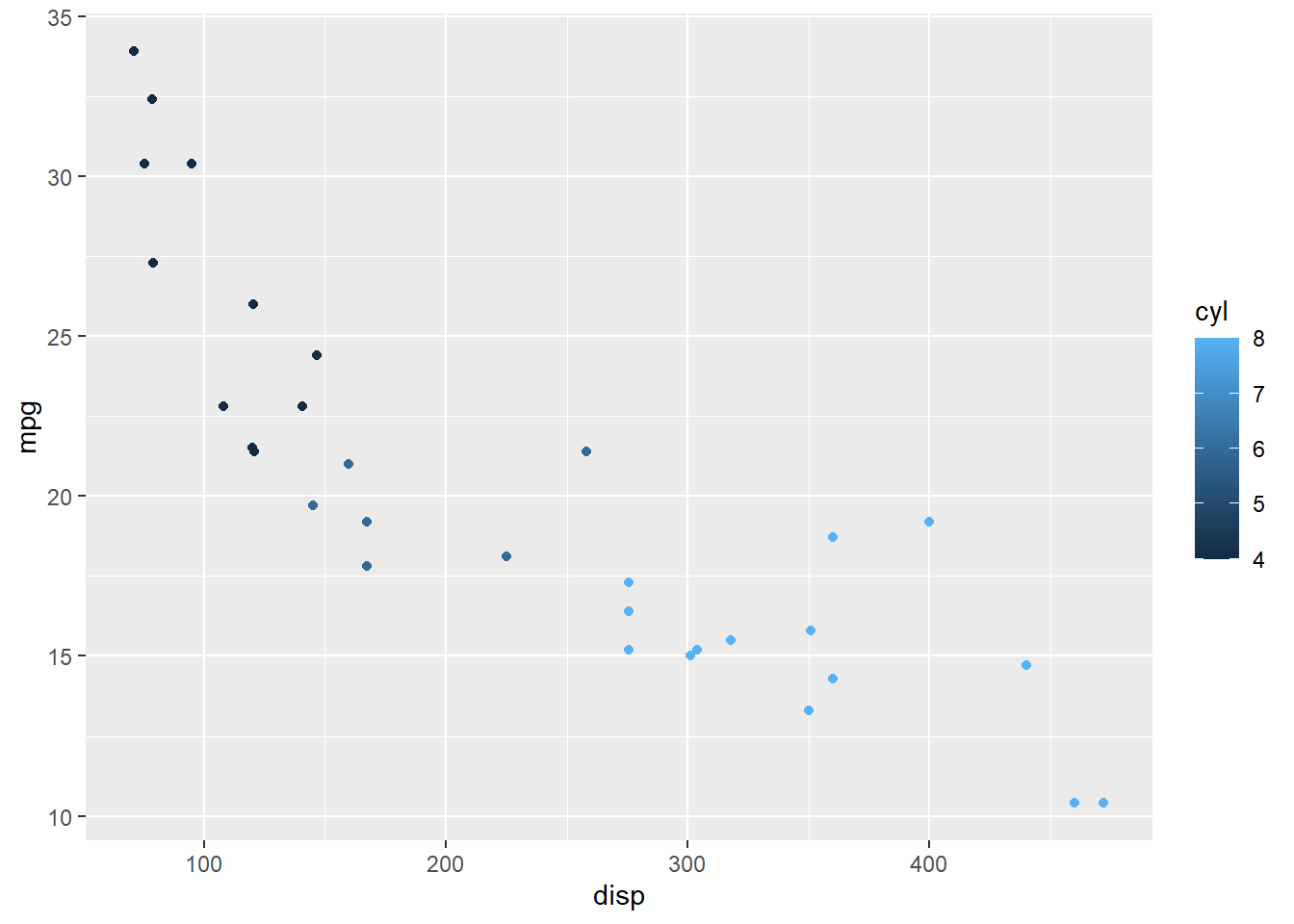
ggplot(mtcars, aes(x=disp, y=mpg,col=factor(cyl)))+geom_point()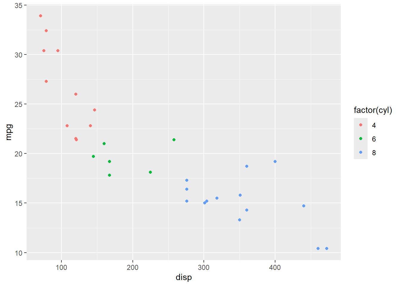 You can see that in the latter case, the colours are much easier to
interpret.
You can see that in the latter case, the colours are much easier to
interpret.
You can change a vector into a factor using the factor()
function, you also have the option of specifying the order of the
levels. Often when you do this it will be part of a data frame, and so
you will want to overwrite the column, like this:
mtcars$cyl <- factor(mtcars$cyl, levels = c('4', '6', '8'))If you only want to use a factor temporarily (like in the example
above) you do not need to overwrite the column, you can use use a
factor() call inline.
Functions
Now that we have seen some different ways to store data, we want to be able to manipulate this data and perform calculations. This is usually done with functions, functions are treated in much the same way as the other objects we have seen so far. To use a function that is in base R (or from a package), we write the functions name, followed by the arguments in parenthesis.
mean(my_vec1) #Mean## [1] 3var(my_vec1) #Variance ## [1] 2.5Every function in R takes some number of arguments. When calling a
function, the arguments are either matched by name or by position. For
example, the function array() takes arguments
data and dim, in the example above, we matched
these arguments by writing array(data = v, dim = c(4,5)) .
Instead, we could have written
v <- 1:20 #vector of data

my_array <- array(v,c(4,5)) #First argument is the data, second argument is the dim vector

print(my_array)
## [,1] [,2] [,3] [,4] [,5]
## [1,] 1 5 9 13 17
## [2,] 2 6 10 14 18
## [3,] 3 7 11 15 19
## [4,] 4 8 12 16 20To find out what the arguments of a function should be, or how to
match arguments correctly, you can use the function help().
In the console, type help() with the name of the function
in the parenthesis. Alternatively, you can also type a question mark
followed by the function name. For example, both
help(array) and ?array return the
following
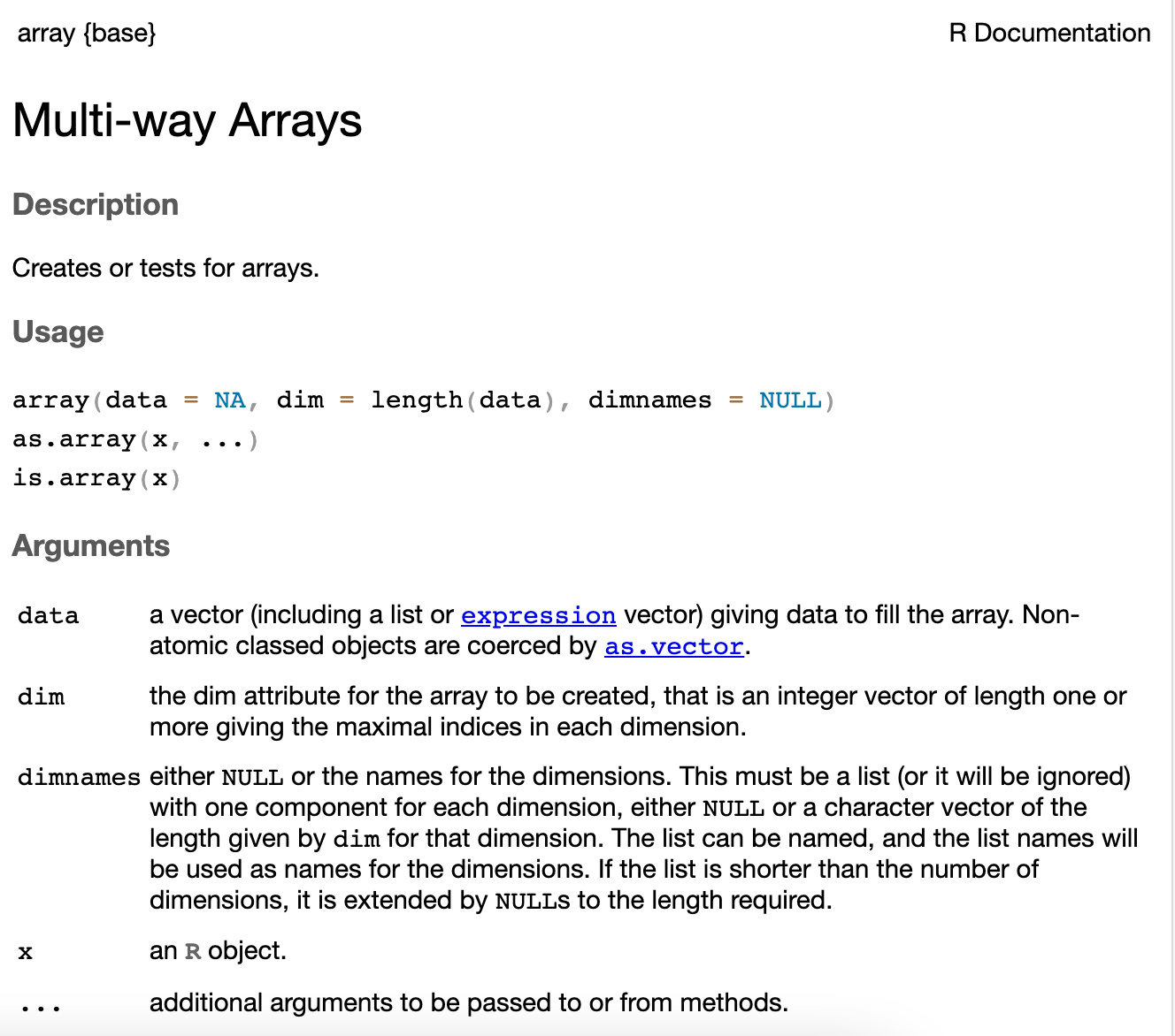
At the bottom of each help page R provides some examples which can be useful to get a better understanding of how the function is used.