Anatomy of RStudio
RStudio is one of many integrated development environments (IDE) that have become the preferred way for users to interact with the R coding language. Many people, especially students who have never used computer code, are introduced to coding in R using RStudio.
I mention this because it is easy to forget that RStudio is an interface that helps us interact with the R programming language. Nothing in RStudio can happen without the separate application R. Similar to the way that social media platforms help us create content on the internet without having to write all of the background code that underlies it, RStudio offers a more user-friendly interface to both gently introduce novice coders to R, and to help expert users code efficiently.
(click here if you have not yet downloaded and installed both R and RStudio)
When you open RStudio on your computer, you will usually see the screen divided into four panes as below (or three panes, Pane 1 might not be shown). I have marked each pane with a number in the screenshot below.
Note: When you open RStudio for the first time, you may only see three panes, two panes on the right, one pane on the left. This is normal, once you open new file, the source pane will appear.

- Pane 1 is the Source pane. Upon opening RStudio, the source pane will either be empty, or will show script files that you left open during the last session.
- Pane 2 is the Console pane, and by default usually contains
three additional tabs that we will not be discussing in this lesson:
- Terminal
- Render
- Background Jobs
- Pane 3 is a customized pane, and by default usually contains the
following 4 tabs:
- Environment*
- History
- Connections
- Tutorial
- Pane 4 is also a customized pane, and by default usually contains
the following 6 tabs:
- Files
- Plots*
- Packages
- Help
- Viewer
- Presentation
Note: The arrangement and content of these panes can be personalized in the “Pane Layout” menu. (Go to View>Panes>Pane Layout)
You can widen or narrow the panes by hovering your cursor over the central border between the left and right panes until the cursor appears as a double-sided arrow and dragging the border left or right. Similarly, you can hover over the border between top and bottom panes until the cursor becomes a double-sided arrow and drag them up or down. This feature is useful when you want to see more of the content of a given pane, such as when you are reading help files or looking at plots in pane 4.
RStudio remembers the pane configuration from your last session, so whatever changes you make to how your panes are arranged, they will still look that way after you close and re-open RStudio.
Aside from the File and Edit menus, the menus at the top of the
screen are bespoke to RStudio. I will not go through each one in detail
here, but I want to point out a few useful things.
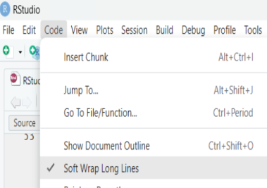
Soft wrap long lines
You may have noticed that when you type in an R script file, the
text just keeps going “off the edge” of the page until you start a new
line (use the return key). If you want all the text in your r script
file to fit within the boundaries on the source pane, you can click on
the Code menu (next to the Edit menu at the top of the screen),
then click “Soft Wrap Long Lines” in the menu. When “Soft Wrap Long
Lines” is turned on, there will be a check mark next to it in the menu,
and the text in the source pane will stay within the boundaries of the
pane, even if you resize the pane by shifting its borders.
RStudio Projects
Before you open a new script file in R, it is a good idea to
open a new or saved project. When you work with project files the
working directory is automatically set to an associated folder where you
can keep the data files that you wish to access for your work.
You can start a new project either by clicking the project
icon  in the top right of the RStudio window and then
selecting “New Project” or by clicking the File menu in the top
left of the RStudio window, and then selecting “New Project”. A new
project wizard dialogue box will appear and offer you the choice to save
your project file to a new or existing directory (folder).
Click on “New Directory”.
in the top right of the RStudio window and then
selecting “New Project” or by clicking the File menu in the top
left of the RStudio window, and then selecting “New Project”. A new
project wizard dialogue box will appear and offer you the choice to save
your project file to a new or existing directory (folder).
Click on “New Directory”.
You should now see the contents of your directory folder in the files
pane (Pane 4). Since you’ve created a new project, the only thing in
your directory folder will be an .Rproj file (your new project file)
like in the below example of the project I created called “Test”.

There are many reasons to use projects files; here are three:
- project files save the ‘environment’ (Pane 3) so that you don’t have to reload your objects every time you open RStudio,
- when you open a project file the directory is automatically set to the folder where it is located,
- if you need to collaborate on an analysis that you’re working on or submit an assignment to your instructor, all of the associated files are together in one place in the directory folder.
You can create a project file in any folder on your computer by choosing the “Existing Directory” option that appears when you open a new project, and selecting an existing folder on your computer (like the folder where your data files are). You will then see the contents of that folder in the files pane (Pane 4).
For more information on projects, watch this ~4 minute video on YouTube: The Basics of Projects in RStudio.
Setting the working directory
You can of course, work in RStudio without using projects by
opening an existing r script file or creating a new one and setting the
working directory manually. When you want to load a data set from an
external file (e.g., an excel file, a csv file, etc.) you need to tell
RStudio how to find those files on your computer and the easiest way to
do that is by setting the directory as the folder where all your files
are kept (Project files assign working directories to their location
automatically. It’s one of the reasons why they are so handy!). The way
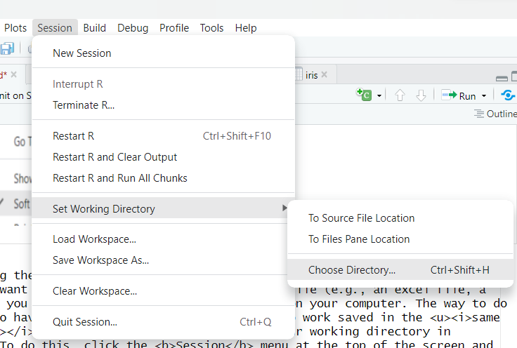
to set a directory is to click the Session menu at the top of the
screen and hover over the menu item “Set working directory” and click
“Choose directory…” from the sub menu that appears.
Note: Remember to save your r script files into the same folder as your working directory so that all associated files are stored together, making them easy to find.
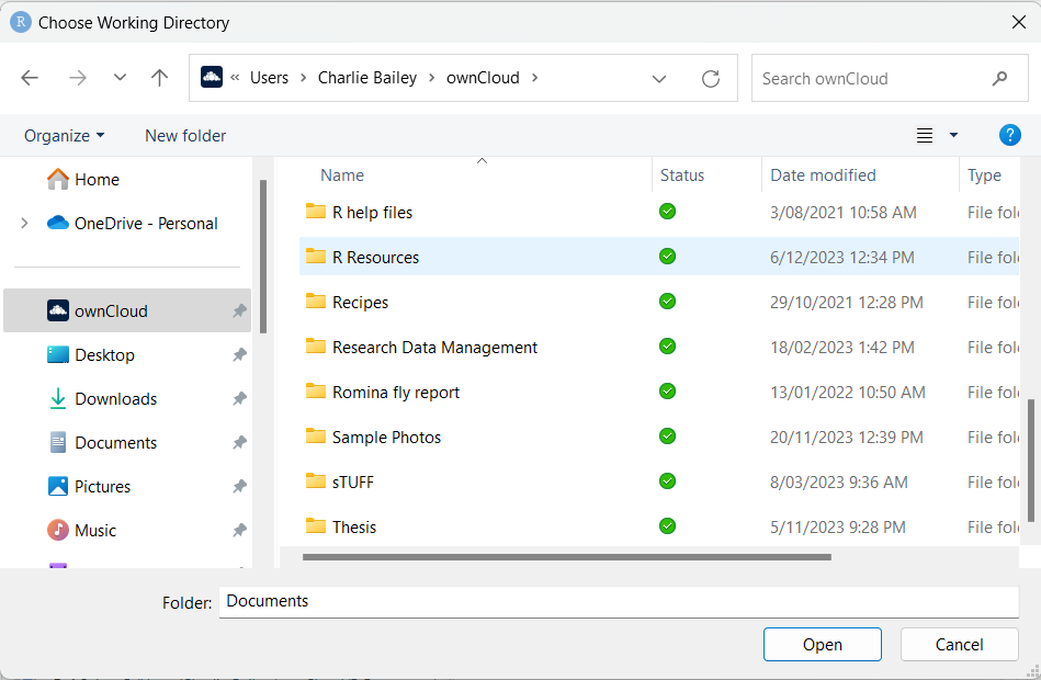
A dialog box will appear for you to navigate to the folder you wish to be your directory. On the left of the dialog box you will see a frame showing “folders” on your computer. If you select a folder on the left, the contents will show on the right. Navigate through by selecting/opening folders until you find the folder where your data files are stored. With the target folder highlighted, you can click on “Open”. Your working directory is now set!
In the below example, I selected OwnCloud from the left-side frame,
then opened successive folders until I found the “R Resources” folder
and clicked it to highlight it, then clicked the “Open” button on the
bottom right.
Now let’s get into the nitty-gritty of the “anatomy” of RStudio and what these parts do.
1: The Source Pane
The Source pane, Pane 1, shows script files that you are working on,
and it can show the contents of some kinds of objects that you’ve
created in the Environment tab of Pane 3 (More on R terminology like
‘objects, vectors, data frames’ here). The
file name of files that are saved appear as black text at the top of the
pane, file names of files that have not yet been saved appear as red
text followed by an asterisk (*). You should save your files often to
avoid losing your work, either by clicking the save icon at the top of
the pane  or by holding the
control button and the ‘s’ key (Ctrl+s,or Command+s for MacOS).
or by holding the
control button and the ‘s’ key (Ctrl+s,or Command+s for MacOS).
Note: If you don’t have any R script files open, pane #1 will collapse upward and pane #2 will extend from top to bottom on the left side of the screen. Pane #1 will reappear once you open a file, or by maximizing the pane by clicking the icon indicated by the yellow arrow.

Let’s open a new R script file by clicking the file menu, then
hovering over “New file”, then clicking on “R Script” in the sub-menu
that appears. Alternately you can use the keyboard shortcut Ctrl+Shift+N
by holding down the ctrl, shift and ‘n’ keys at the same time
(Command+Shift+N for MacOS).
In your new r script file, type or copy/paste the following (text in the below grey box):
DataFrame <- data.frame(ID = c(1, 2, 3, 4, 5),
                  var1 = c('a', 'b', 'c', 'd', 'e'),
                  var2 = c(1, 1, 0, 0, 1))
With your cursor positioned anywhere within the three lines of code
(but not highlighting any text), click the “Run” button
 at the top of the pane, or
alternatively, hold down the control and enter keys at the same time
(Ctrl+Enter, or Command+Return for MacOS).
at the top of the pane, or
alternatively, hold down the control and enter keys at the same time
(Ctrl+Enter, or Command+Return for MacOS).
Congratulations, you just created a data frame object. Let’s take a second to name the parts of the code you just executed.
- “DataFrame” is the name of the object, you can see it listed in the environment pane.
- <- this symbol assigns the code on the right-hand side of the arrow to the object name on the left-hand side of the arrow
data.frame()is a function that creates an object of class “data.frame”- ID, var1, and var2 are the names of the columns of the data frame.
c()is the concatenate function. It connects the vectors between the parentheses into the assigned column of the data frame.
For more information about data frames, see the Data Frames section
of R Basics
Note: If you want to make notes in your r script file, you must preceed your notes with the hash symbol (#). For example:
DataFrame <- data.frame(ID = c(1, 2, 3, 4, 5),   # Making a 'dummy dataset'
                  var1 = c('a', 'b', 'c', 'd', 'e'),
                  var2 = c(1, 1, 0, 0, 1))
Note: The “quoted” text that follows the hash symbol appears in green and is not executable by R, meaning that R will ignore anything in green when it runs your code. Taking notes this way can be a really useful way to keep track of what code you wrote and why and act as a reminder to you when you haven’t used RStudio in a while.
You will see that the object called “DataFrame” has
appeared in pane 3 in the Environment tab under the heading “Data”. On a
new line, type the following and click the run button.
View(DataFrame)A new window should appear in the source pane showing the data frame object that you just created. You can also view an object from the environment pane by clicking on its name. It will then appear in the source pane.
Note: If you mispell or change the case of function names and objects in R, you will get an error message in the console pane. This is because coding in R is case-sensitive. It is important to remember this when creating objects; use short words that you can easily type repeatedly. This is also important to remember when using functions. A function like “View”, typed in all lower case letters “view”, doesn’t mean anything in the base R language. BTW, whenever anyone makes mention of “base r” they are referring to functions that come included with the r application.
2: The Console Pane
The console pane, Pane 2, shows outputs or results of commands that you execute in either your R script file in the source pane, or directly in the console window of the console pane. Try typing 2+3 on a new line in your r script file and then clicking “run” or hold down “Cntrl + Enter”.
2+3## [1] 5You will see the result, 5, in the console pane.
As another example, try typing “pi” on a new line in your r script file in the source pane, then “Cntrl + Enter”.
pi## [1] 3.141593R returns the irrational number “pi”, 3.141593, in the console pane.
The console pane is also where you will see error or warning massages
to alert you about things like syntax errors in your code or warnings
about limitations of statistical inference (for example). These messages
appear as red text in the console. Errors halt the execution of your
command(s), while warnings do not. You can highlight text in the console
for confusing error messages to copy them and then paste them into an
internet search engine and search for help to solve the error. For
example, the error in the screenshot below occurred because the working
directory was not set, and RStudio could not locate the data file in the
read.csv() function.

We will not be
covering the other three tabs in the console pane in this lesson
(Terminal, Render, and Background Jobs).
3. The Environment pane
Pane 3, which I will call the Environment pane, is most useful for viewing a list of the objects you’ve made. Let’s call a data set that is saved in R called “iris”.
irisThe “iris” data set contains measurements taken from the flowers of
three species of Iris. Because this data set is stored within the R
application, you do not need a function to call it. However, if you want
to use it in other functions, you will need to load it into your
environment. We will do that now with the data()
function.
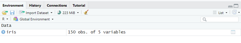
data(iris)iris now appears in the environment pane (Pane 3) with a short description of its size, 150 observation (obs.) of 5 variables. The number of observations tells you how many rows are in the data frame, the number of variables tells you the number of columns in the data frame.
The environment pane can tell you more about the iris data frame object than just its name. Click on the blue toggle to the left of the object named “iris”.
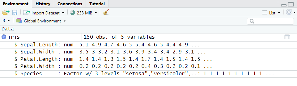
iris now appears in the environment pane as an expanded list describing each variable by name, then class, and gives a truncated list of the first 10 values in each column. You can see that the data frame includes numerical values and categorical values (factors).
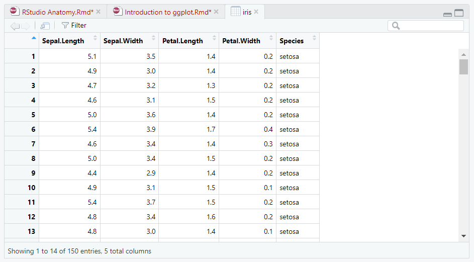
We’ll do one last thing with the iris data frame. Click on the word iris in the environment pane. The iris data frame opens in the source pane as its own tab.
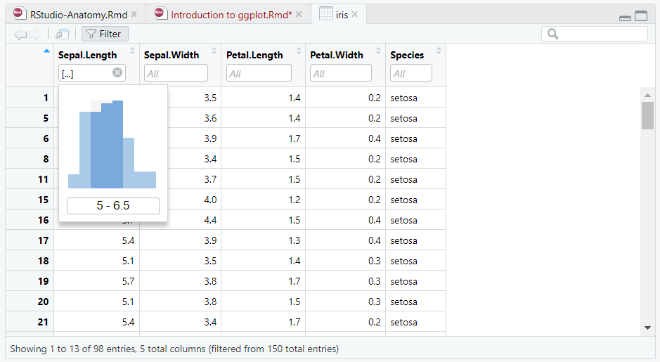
Just above the data frame, you will see the filter icon
 . If you click it, you will
see a rectangle below each column name containing the word “All”. If you
click the rectangle below the name “Sepal.Length”, a histogram will
appear showing the distribution of the data contained in the column. You
can click, or click-and-drag in the histogram to choose only some sepal
lengths, and the data set will become filtered to show only the rows
that contain the sepal lengths that you highlighted in the histogram. If
you click the rectangle below the categorical variable “Species”, you
will see a list of the three species factors from which you can filter
the data set by iris species.
. If you click it, you will
see a rectangle below each column name containing the word “All”. If you
click the rectangle below the name “Sepal.Length”, a histogram will
appear showing the distribution of the data contained in the column. You
can click, or click-and-drag in the histogram to choose only some sepal
lengths, and the data set will become filtered to show only the rows
that contain the sepal lengths that you highlighted in the histogram. If
you click the rectangle below the categorical variable “Species”, you
will see a list of the three species factors from which you can filter
the data set by iris species.
The environment saves all the objects that you make during an RStudio session. That is to say, even if you are executing code in more than one r script file in the same RStudio session, all the objects that you create will be saved into one environment pane until you quit the RStudio application, at which point the Environment will be cleared (Unless the environment you created is associated with a project file, in which case the environment will be saved).
I mention this for two reasons:
- If you leave an R script file open in the source pane when you quit RStudio, the source pane will appear as you left it the next time you open RStudio. However, the environment pane will be empty. Objects you saved into the environment during your previous RStudio session are cleared from the environment when you quit the application. You will need to re-run your scripts every time you open RStudio so that RStudio can save your objects into the environment pane again.
If you create a project file, you will not have to re-run your scripts to save them to the environment; the project file keeps them saved.
- The environment can get cluttered with objects if you are working in
RStudio for a long time. If you want to clear the environment for any
reason, you can do so by clicking the “clear objects from the workspace”
icon
 at the top of the
environment pane. This will clear all objects from the environment, so
you’ll have to run the code you are working on again to re-save them to
the environment.
at the top of the
environment pane. This will clear all objects from the environment, so
you’ll have to run the code you are working on again to re-save them to
the environment.
4. The Plot/Help pane
The fourth and final pane of RStudio is possibly the most useful in the context of user-interface experience, as you can see both your working r script file in the source pane at the same time as you can see plots you create, or help files that you need to read as you are coding. I’m going to go through each tab one at a time, but I will not be talking about the Viewer and Presentation tabs in this lesson.
Files
The files tab allows you to see files in a designated folder on your
computer. Remember that folder where you saved your data files? Once
that folder is set as your working directory, you can easily view this
folder in the “files” tab. If you can’t already see the contents of your
working directory in the files tab, click on the “More” icon
 and select “Go to working
directory” from the menu that appears.
and select “Go to working
directory” from the menu that appears.
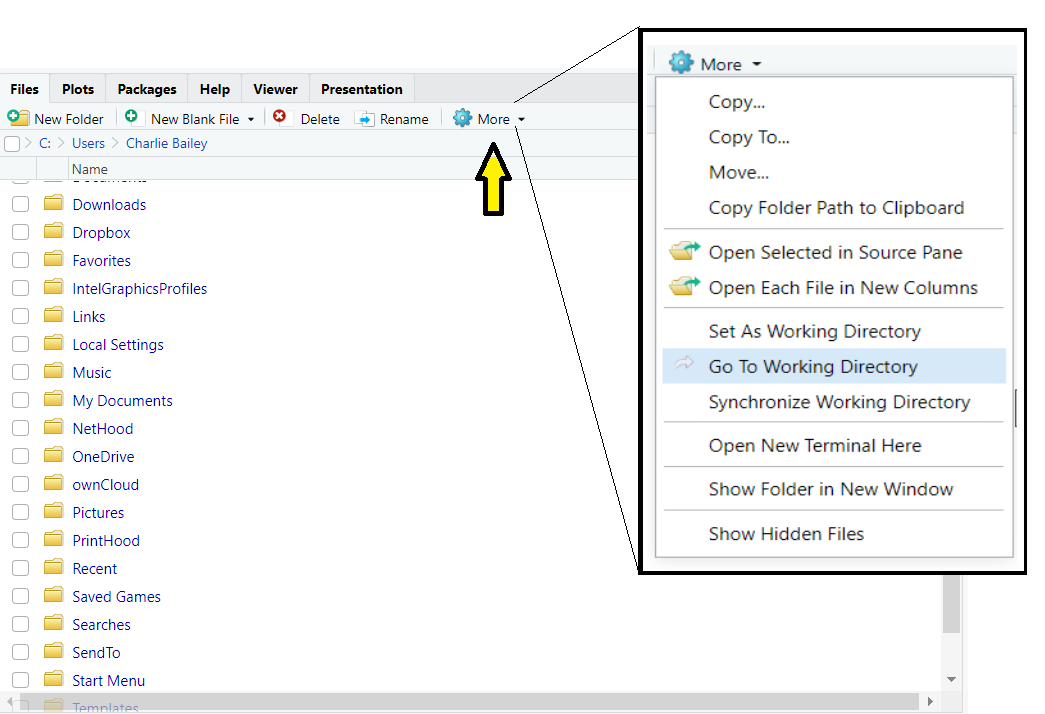
The files tab now shows the contents of your working directory.
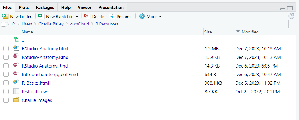
This is useful because it lets you see the files that R will look for when reading data (see here), or files that you have created (e.g., when saving plots).
Plots
The “plots” tab is where the plots you generate in your r script will appear. Let’s use the iris data frame to plot a scatter-plot that shows the relationship between sepal length and sepal width.
Type the following code, which includes the data()
function from before to load the iris data set into the environment. The
plot() function is included in base r and allows the
printing of a number of plot types. The code I used “iris$sepal.length”
is shorthand to call the column “sepal.length” from the data frame
“iris”. You can do this with any data frame object by typing the object
name, followed by the $ symbol, and then the column name, without any
spaces. There is more information on creating basic plots here, or more advanced plots here.
data(iris)
plot(iris$Sepal.Length ~ iris$Sepal.Width)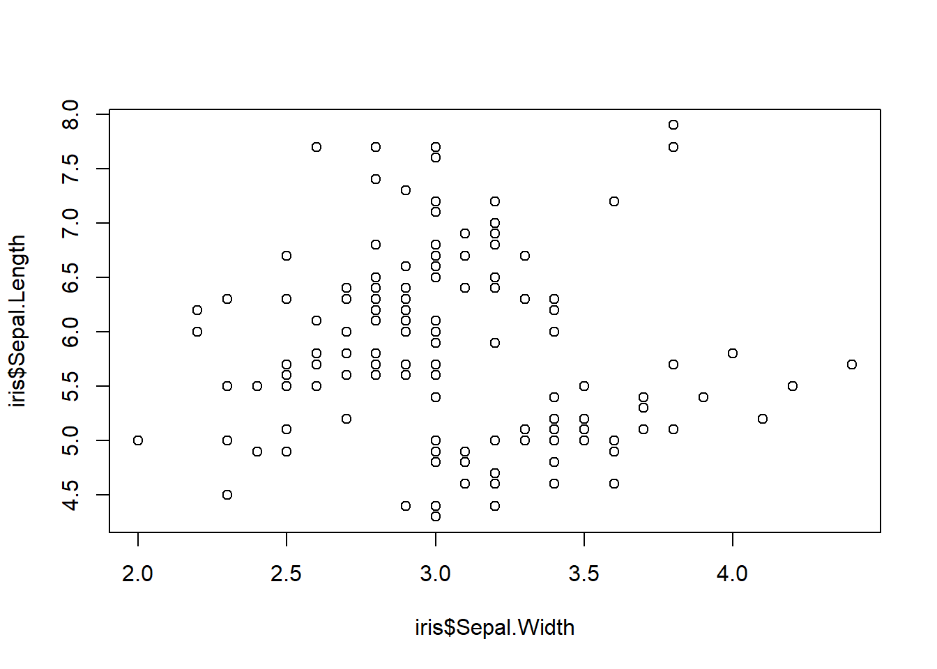
The above plot should appear in the Plot/Help pane.
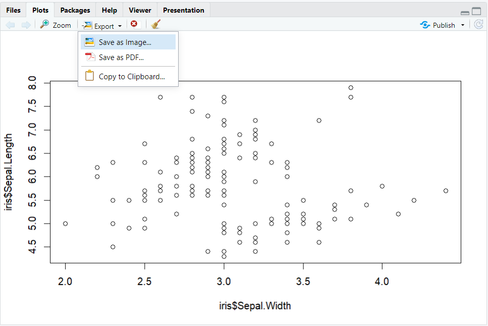
You can save plots from the Plot/Help pane for use in other apps such as
Microsoft Word by clicking the export icon
 and saving the plot either as
an image or as a pdf, or by copying it to the clipboard (to be pasted
elsewhere).
and saving the plot either as
an image or as a pdf, or by copying it to the clipboard (to be pasted
elsewhere).
Packages
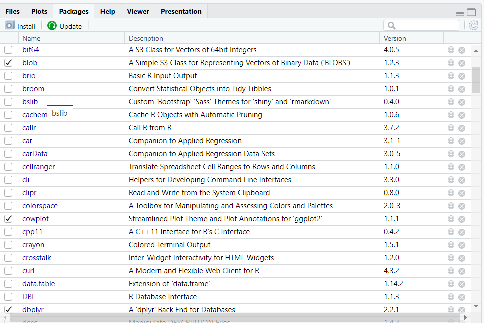
The packages tab of the Plots/Help pane shows a list of packages that
are installed in RStudio and shows whether those packages are loaded by
displaying a check-mark next to the package name.
See the R Packages page for more information on installing and using packages.
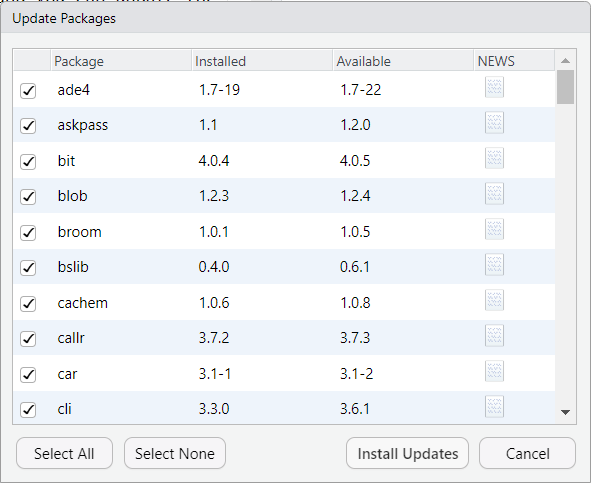
New versions of packages get released from time to time, and you can
update the packages in the packages tab by clicking the Update icon.
 This will open a dialog box
showing all of the packages you have installed that have updates
available. You can choose to update all of them, or choose which to
update by clicking the check boxes next to each package name.
This will open a dialog box
showing all of the packages you have installed that have updates
available. You can choose to update all of them, or choose which to
update by clicking the check boxes next to each package name.
Help
The help tab of the Plots/Help pane displays help files for specific functions and packages. You can call a help file for any function, if that function’s package is installed and loaded in RStudio, by typing a ? in front of the function in either an r script file, or directly into the console pane on the bottom line, like so.
?hist
Running the above code should open the help file for the
hist() function in the help tab of the Plots/Help pane.
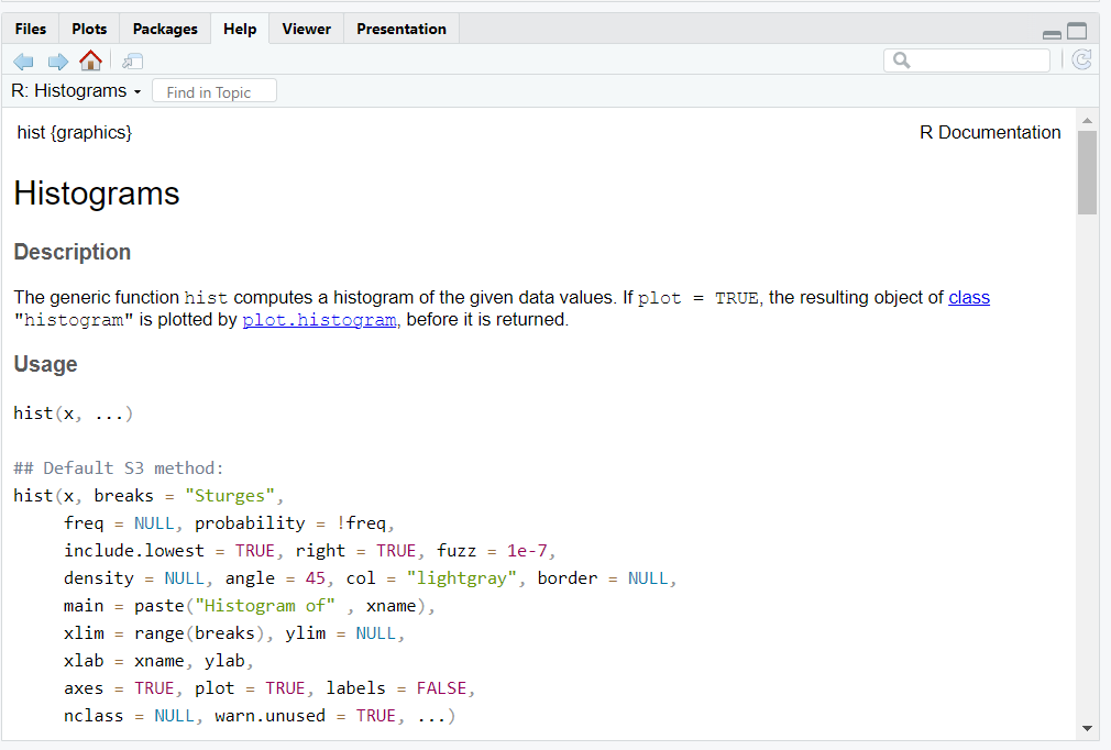
At the top left of the help file, you will see the function name followed by its package in curly brackets {}.
Each help file has the same sections:
- Title - Gives a full name to the function.
- Description - Tells you what the function is used for, and sometimes, notes about its usage.
- Usage - Gives an example of how the arguments are ordered by default in the function.
- Arguments - Describes each of the arguments of the function including class requirements and additional links with further information.
- Details - Additional notes about how the functions operates, including tips and sometimes troubleshooting.
- Value - Describes the output of the function, and may further describe elements of the output values.
- References - Bibliographic information to publications that discuss the use of the function.
- See also - Links to associated help files to aid in the use of the function.
- Examples - Examples of how to use the function.