Common Probability Distributions in R

Probability distributions describe the possible behaviours of common random phenomena, mathematically. They encode both how the values of the random variables are distributed and spread out, and probability of each outcome. There are two main types of probability distributions: discrete and continuous. MATH260/MATH460 covers many common probability distributions in reasonable depth.

R employs a consistent method for handling probability distributions, with each distribution featuring four functions identified by prefixes d, p, q, or r for probability function, distribution function, quantile function and random sample respectively.

Every probability distribution relies on one or more parameters that need to be explicitly defined when utilizing these functions. E.g, For normal distributions, the parameters are:

• mean
• sd-standard deviation

For a random variable \(X\), which follows normal distribution with mean=\(\mu\) and standard deviation = \(\sigma\), we write \(X \sim N(\mu, \sigma^2)\).

The functions associated with normal distributions are:

Prefix	Function	Example
d	Probability function	dnorm
p	Distribution function	pnorm
q	Quantile function	qnorm
r	Random sample	rnorm

The probability function(prefix d) calculates the probability density function(pdf) for continuous distributions and the probability mass function(pmf) for discrete distributions. It determines the probability associated with a given value of \(x\) and the specified parameters.

The distribution function (prefix p) gives the probability that a random variable X is less than or equal to a given value.

\(F_X(x) =P(X \leq q)\), for all value of x.

The lower.tail Parameter : The \(p\) (distribution) functions have an optional parameter lower.tail, which can have the values TRUE or FALSE. The default is lower.tail =TRUE, which calculates \(F_X(x) =P(X \leq q)\). When lower.tail = FALSE, we calculate the upper tail,

\[1 - F_X(q) =1- P(X \leq q) = p(X>q)\]

Quantile function (prefix q) is used to find the value in a probability distribution that corresponds to a specific probability. i.e, it helps you determine the cutoff point below which a certain percentage of the data falls. For any random variable \(X\) the \(p^{th}\) quantile of \(X\) for \(0 < p < 1\) is the value \(x\) such that \[P(X ≤ x) = F_X (x) = p\]

The \(q\) (distribution) functions also have an optional lower.tail parameter. If lower.tail = FALSE the \(q\) function computes, for a given \(p\), the value \(x\) such that \[P(X > x) = 1 − F_X (x) = p\] Random function (prefix r) generates samples of random numbers associated with the specified distribution.

We will look at various probability distributions and demonstrate how \(R\) functions can be used in each case.. Detailed examples of the normal distribution for continuous cases and the binomial distribution for discrete cases are provided.

Continuous probability distribution

Normal distribution

Normal distribution is a probability distribution in which the values are symmetrically distributed around the mean. The parameters are mean=\(\mu\) and standard deviation = \(\sigma\).

Let X be random variable which follows normal distribution with mean=\(\mu\) and standard deviation = \(\sigma\), then we write \(X \sim N(\mu, \sigma^2).\)

Note: The standard normal distribution is the normal distribution with \(\mu =1\) and \(\sigma = 1\).

Mean and variance of normal distribution:

• mean = \(\mu\)

• variance = \(\sigma^2\)

The functions associated with the normal distribution are used as follows

dnorm(x= , mean= , sd= )
pnorm(q= , mean= , sd= , lower.tail= )
qnorm(p= , mean= , sd= , lower.tail= )
rnorm(n= , mean= , sd= )

Graph of probability density function of normal distribution with different parameters:

See figure code

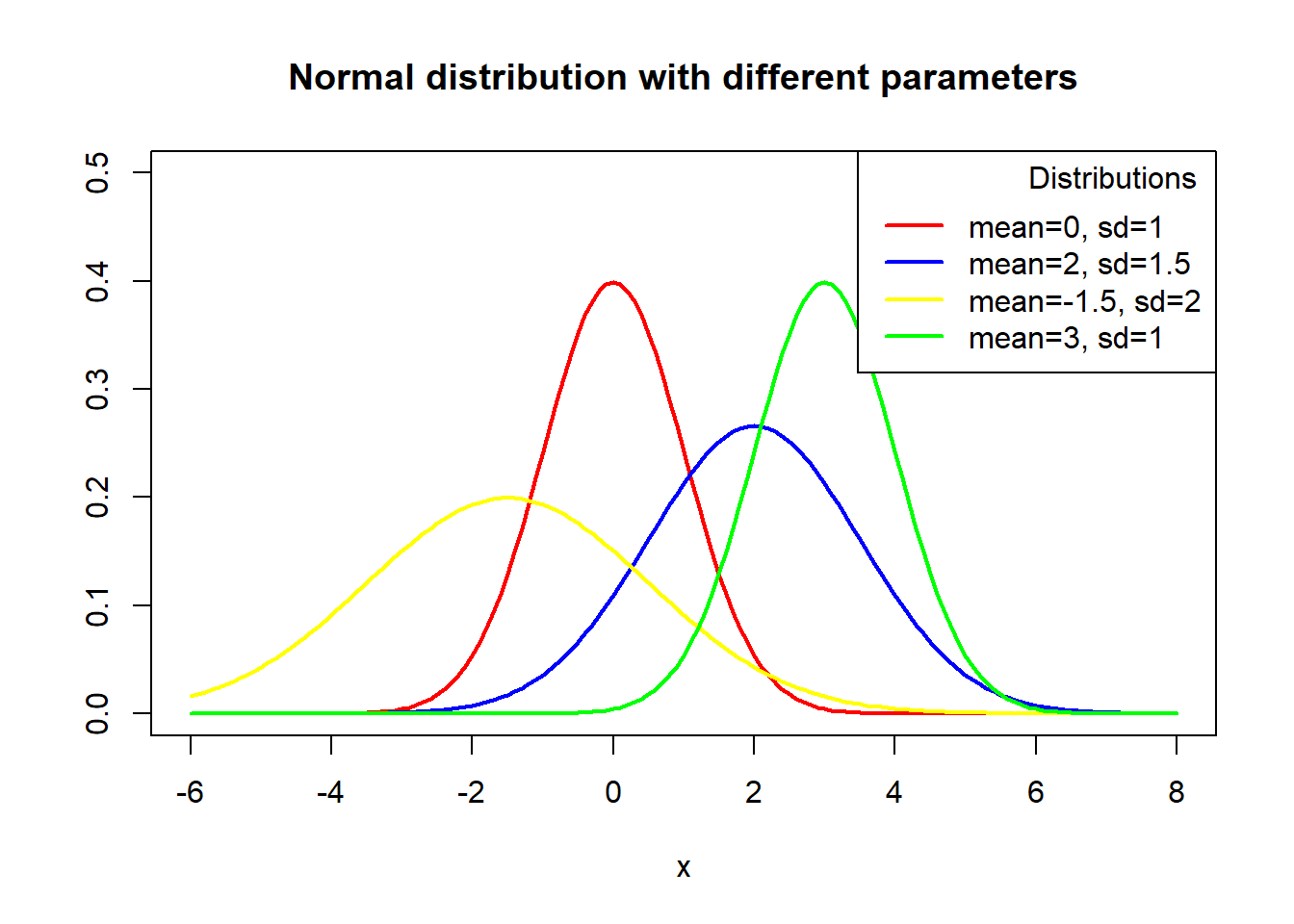
x <- seq(-6, 8, 0.1)
plot(x, dnorm(x, mean = 0, sd = 1), type = "l",
     ylim = c(0, 0.5), ylab = "", lwd = 2, col = "red", main = "Normal distribution with different parameters")
# Mean 2, sd 1.5
lines(x, dnorm(x, mean = 2, sd = 1.5), col = "blue", lty = 1, lwd = 2)
# Mean -1.5, sd 2
lines(x, dnorm(x, mean = -1.5, sd = 2), col = "yellow", lty = 1, lwd = 2)
# Mean 3 , sd 1

lines(x, dnorm(x, mean = 3, sd = 1), col = "green", lty = 1, lwd = 2)

# Adding a legend
legend("topright", legend = c("mean=0, sd=1", "mean=2, sd=1.5", "mean=-1.5, sd=2", "mean=3, sd=1"), col = c("red", "blue", "yellow", "green"),
       title = "Distributions",
       title.adj = 0.9, lty = 1, lwd = 2)

Example

Suppose \(X\) is normally distributed with \(mean = 2.5\) and \(sd =0.75\), we write \(X \sim N(2.5, 0.75^2)\).

• Plot the density function and compute the value of probability density at \(x = 1.5\)

answer

# Plot the probability density
plot(function(x) dnorm(x, mean=2.5, sd=0.75), 0, 5)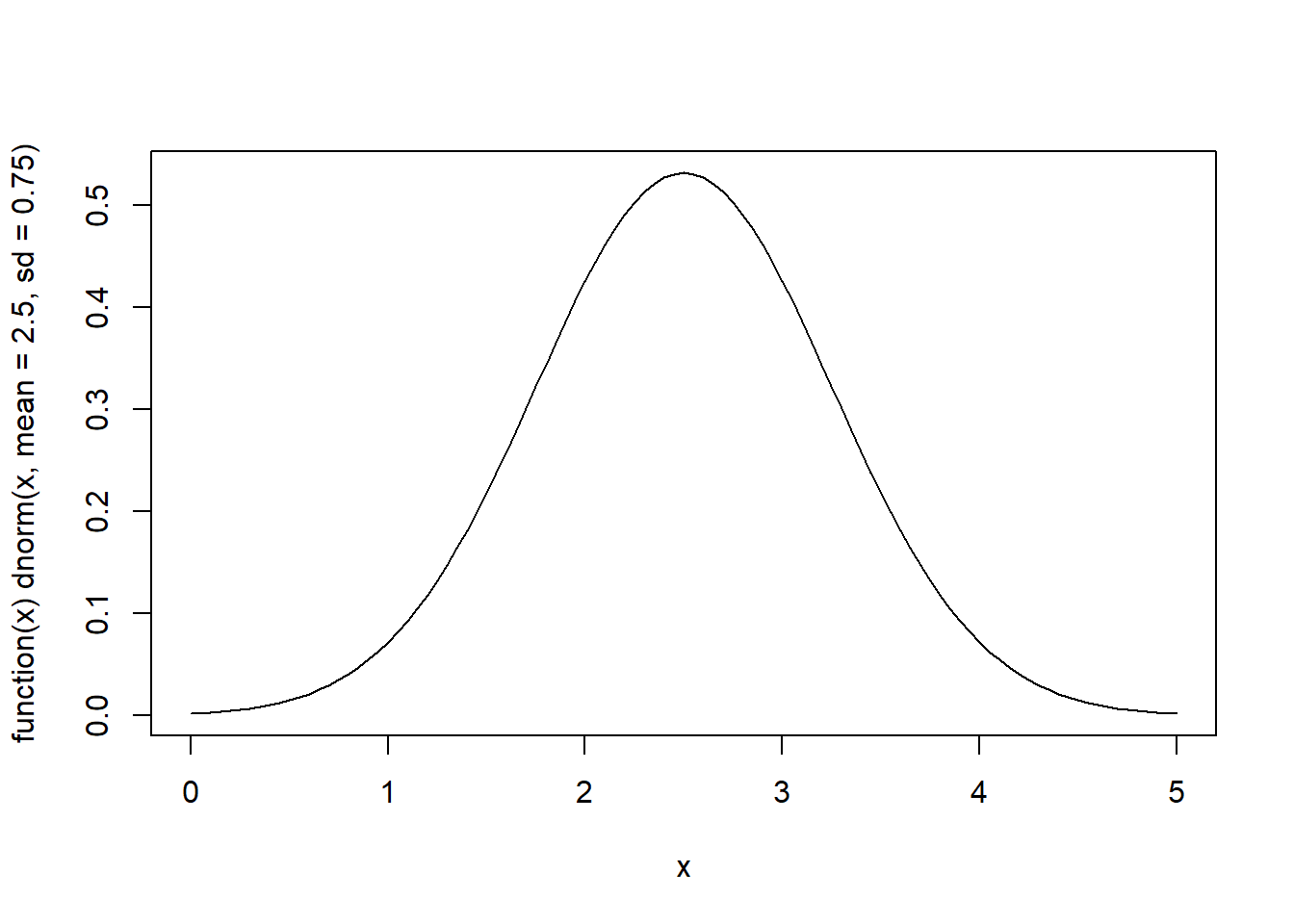

# P(X=1.5)
dnorm(x=1.5, mean=2.5, sd=0.75)

## [1] 0.2186801

• Plot the cumulative distribution function and compute \(P(X < 1.75)\), \(P(1 < X < 3)\), \(P(X < 4)\).

answer

# Plot the cumulative distribution function
plot(function(q) pnorm(q, mean=2.5, sd=0.75), 0, 5)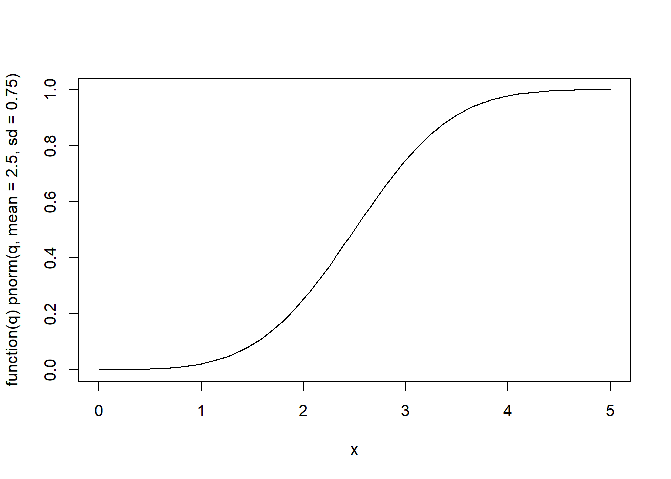

#P(X < 1.75)
pnorm(q=1.75, mean=2.5, sd=0.75)

## [1] 0.1586553

# P(1 < X < 3)
p1 = pnorm(q=1, mean=2.5, sd=0.75)
p2 = pnorm(q=3, mean=2.5, sd=0.75)
p1 - p2

## [1] -0.7247573

# Alternatively we can use
diff(pnorm(q=c(1,3), mean=2.5, sd=0.75))

## [1] 0.7247573

# P(X < 4)
pnorm(q=4, mean=2.5, sd=0.75, lower.tail=FALSE)

## [1] 0.02275013

• Find the value of \(x\) such that \(P(X \leq x) = 0.90\).

answer

qnorm(p=0.90, mean=2.5, sd=0.75)

## [1] 3.461164

# If we want to find x such that P(X > x) = 0.90

qnorm(p=0.90, mean=2.5, sd=0.75, lower.tail = FALSE)

## [1] 1.538836

• Generate 1000 normal random numbers with mean = 2.5 and sd=0.75, plot their histogram and the probability density function.

answer

# generate 1000 normal random numbers
x <- rnorm(1000, mean=2.5, sd=0.75)

#plot the histogram
hist(x, probability=TRUE, ylim = c(0,0.6))

# generate xx values 
xx <- seq(min(x), max(x), length=100)

# add the density function
lines(xx, dnorm(xx, mean=2.5, sd=0.75))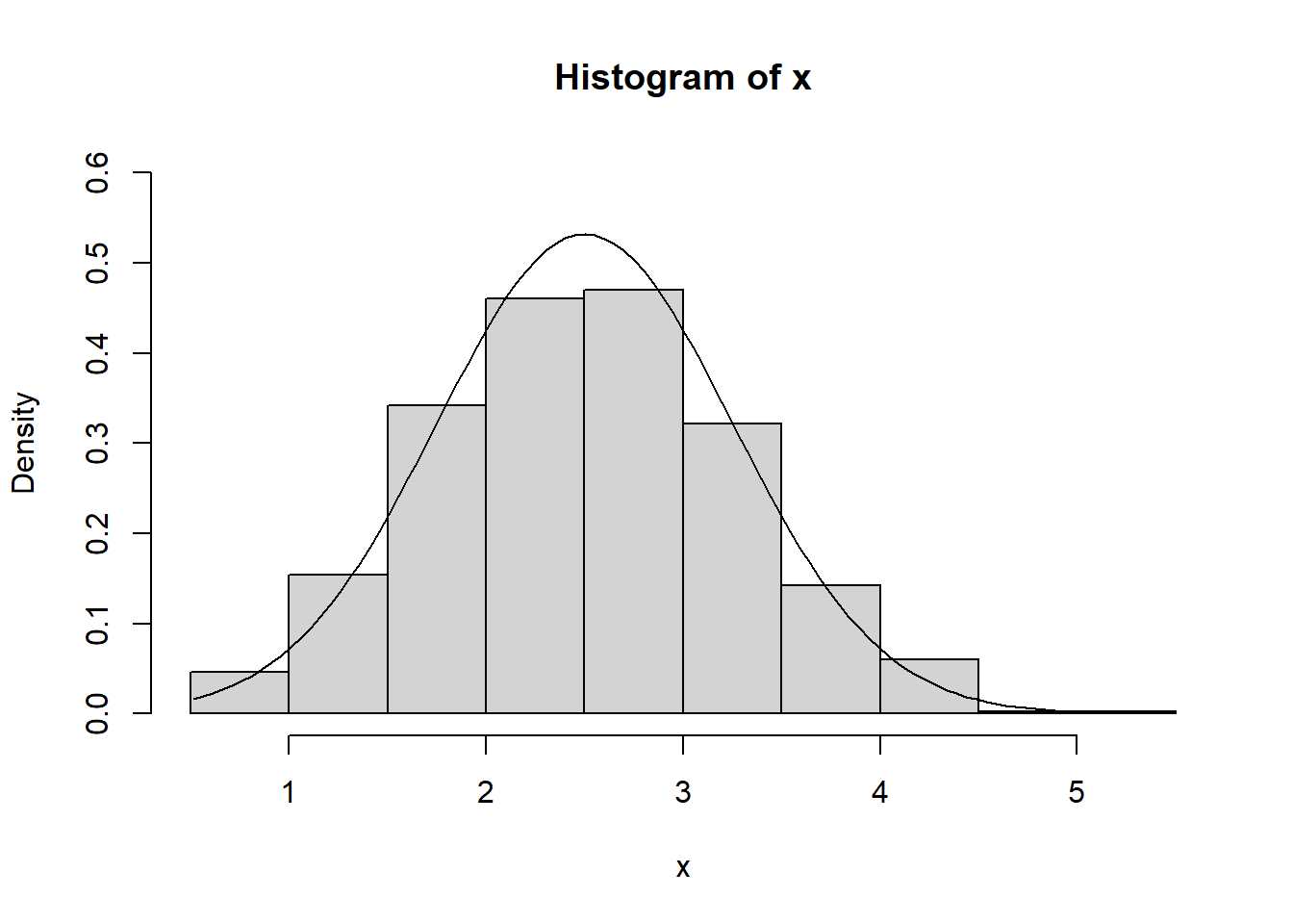

Uniform distribution

Uniform distribution is a probability distribution where each possible outcome has an equal chance of occurring. The parameters of the uniform distribution are the maximum (Max) and minimum (Min) values of the interval. We write \(X \sim U(a,b)\).

Mean and variance of uniform distribution:

• mean = \(\frac{a+b}{2}\)

• var = \(\frac{(b-a)^2}{12}\)

The functions associated with the uniform distribution are used as follows;

dunif(x= , min= , max= )
punif(q= , min= , max= , lower.tail= )
qunif(p= , min= , max= , lower.tail= )
runif(n= , min= , max= )

Graph of uniform probability density;

See figure code

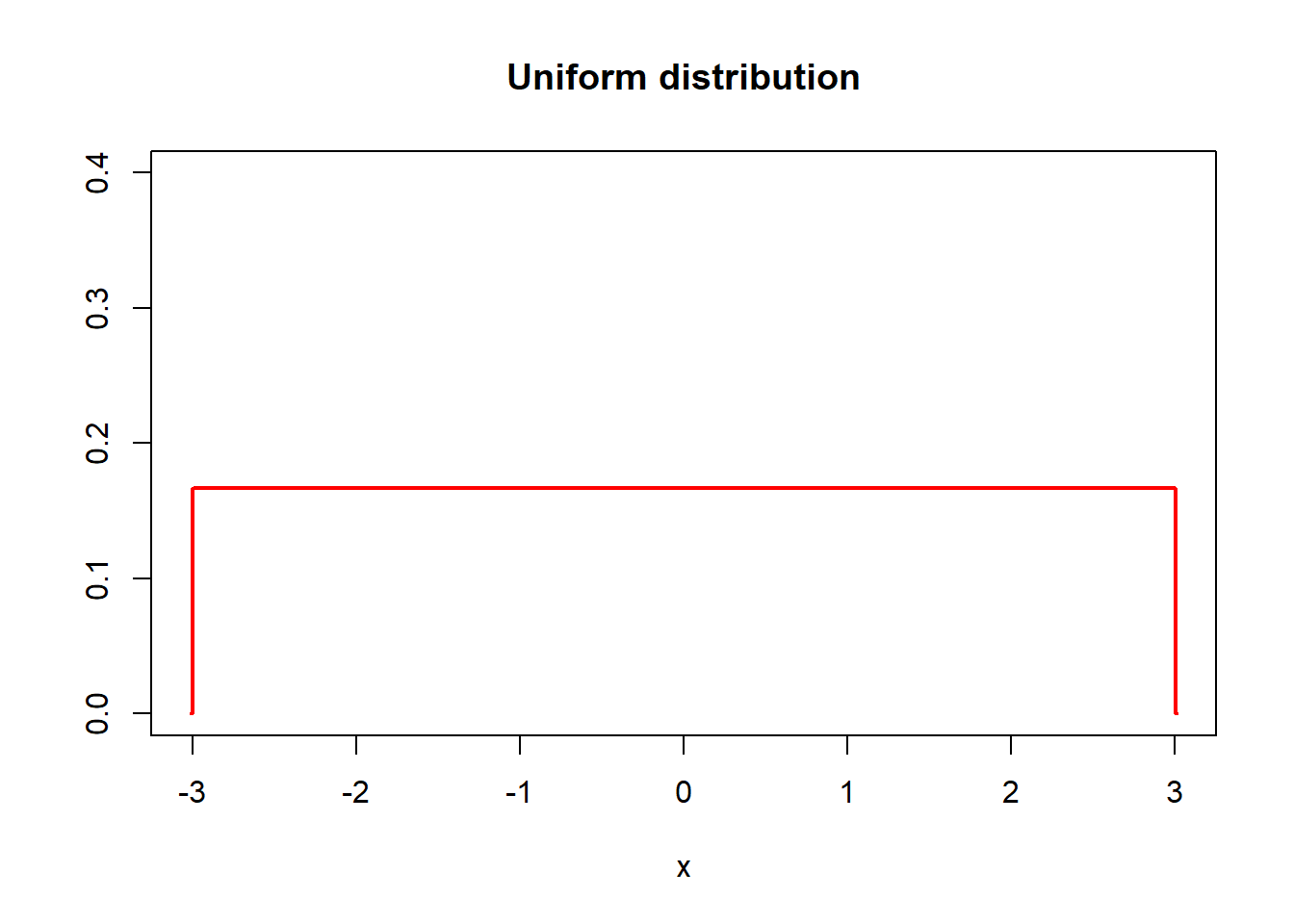
# Define x-axis
x <- seq(-3.01, 3.01, length=1000)

#Plot uniform distribution
plot(x, dunif(x, min= -3, max= 3), ylim= c(0,0.4), ylab = "", type = "l",  lwd = 2, main = "Uniform distribution", col = "red")

Exponential Distribution

The exponential distribution is a continuous probability distribution that models the time until the next event in a sequence of independent events. Exponential distribution has one parameter, known as rate parameter, \(\lambda\) which is rate of event per unit time. If \(\beta\) is the average time until the event occurs, \(\lambda = \frac{1}{\beta}\).

Let \(X\) be random variable which follows an exponential distribution with rate \(\lambda\), we write \(X \sim Exp(\lambda)\).

Mean and variance of exponential distribution:

• mean = \(\frac{1}{\lambda}\)

• Variance = \(\frac{1}{\lambda^2}\)

The functions associated with the exponential distribution are used as follows:

dexp(x= , rate= )
pexp(q= , rate= , lower.tail= )
qexp(p= , rate= , lower.tail= )
rexp(n= , rate= )

Graph of probability density function of exponential distributions with different parameters:

See figure code

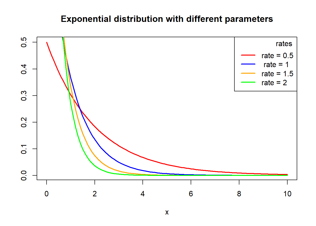
x <- seq(0, 10, 0.1)
plot(x, dexp(x, rate = 0.5), type = "l",ylab = "", lwd = 2, col = "red", main = "Exponential distribution with different parameters")

lines(x, dexp(x,rate =1 ), col = "blue", lty = 1, lwd = 2)

lines(x, dexp(x,rate = 1.5), col = "orange", lty = 1, lwd = 2)


lines(x, dexp(x, rate = 2), col = "green", lty = 1, lwd = 2)

# Adding a legend
legend("topright", legend = c("rate = 0.5", " rate = 1", "rate = 1.5", "rate = 2"), col = c("red", "blue", "orange", "green"),
       title = "rates",
       title.adj = 0.9, lty = 1, lwd = 2)

Gamma Distribution

Gamma Distribution is a continuous probability distribution widely used to model the time until the \(\alpha^{th}\) event to occur. Gamma distribution has two parameters \(\alpha\)- shape parameter and \(\beta\)- scale parameter.

Note: When \(\alpha=1\), Gamma distribution is an exponential distribution.

Note: Sometimes the Gamma distribution has a different parametrizeation, so be careful that you are using the parameters you intend to.

Let X be random variable which follows Gamma distribution with parameters \(\alpha\) and \(\beta\), we write \(X \sim Gamma(\alpha, \beta)\).

Mean and variance of Gamma distribution:

• mean = \(\alpha \beta\)

• Variance = \(\alpha \beta^2\)

The functions associated with the Gamma distribution are used as follows:

dgamma(x= ,shape= ,scale=)
pgamma(q= ,shape= ,scale= ,lower.tail= )
qgamma(p= ,shape= ,scale= ,lower.tail=)
rgamma(n= ,shape= ,scale=)

Graph of probability density function of Gamma distributions with different parameters:

See figure code

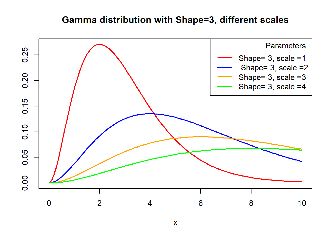
x <- seq(0, 10, 0.1)
plot(x, dgamma(x, shape = 3, scale = 1), type = "l", ylab = "", lwd = 2, col = "red", main = "Gamma distribution with Shape=3, different scales")

lines(x, dgamma(x, shape = 3, scale = 2), col = "blue", lty = 1, lwd = 2)

lines(x, dgamma(x, shape = 3, scale = 3), col = "orange", lty = 1, lwd = 2)


lines(x, dgamma(x, shape = 3, scale = 4), col = "green", lty = 1, lwd = 2)

# Adding a legend
legend("topright", legend = c("Shape= 3, scale =1", " Shape= 3, scale =2", "Shape= 3, scale =3", "Shape= 3, scale =4"), col = c("red", "blue", "orange", "green"),
       title = "Parameters",
       title.adj = 0.9, lty = 1, lwd = 2)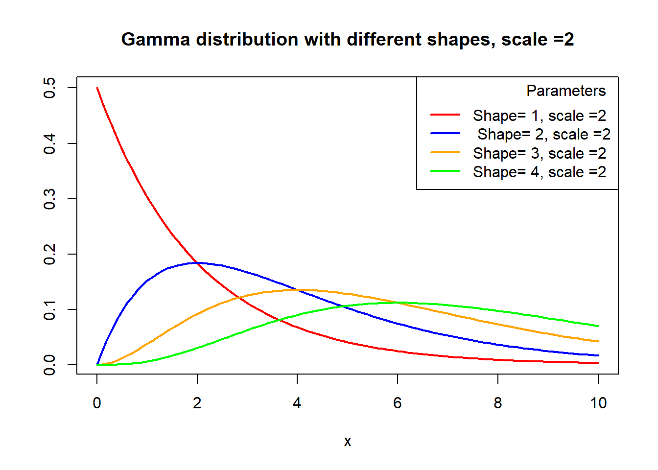

See figure code

x <- seq(0, 10, 0.1)
plot(x, dgamma(x, shape = 1, scale = 2), type = "l", ylab = "", lwd = 2, col = "red", main = "Gamma distribution with different shapes, scale =2")

lines(x, dgamma(x, shape = 2, scale = 2), col = "blue", lty = 1, lwd = 2)

lines(x, dgamma(x, shape = 3, scale = 2), col = "orange", lty = 1, lwd = 2)


lines(x, dgamma(x, shape = 4, scale = 2), col = "green", lty = 1, lwd = 2)

# Adding a legend
legend("topright", legend = c("Shape= 1, scale =2", " Shape= 2, scale =2", "Shape= 3, scale =2", "Shape= 4, scale =2"), col = c("red", "blue", "orange", "green"),
       title = "Parameters",
       title.adj = 0.9, lty = 1, lwd = 2)

Beta Distribution

The beta distribution is a continuous probability distribution that models random variables with values falling inside a finite interval. The standard beta distribution uses interval \([0,1]\), which is ideal for modeling proportions or probabilities. It has two shape parameters, \(m\) = shape1 and \(n\)=shape2, which controls the shape of the distribution.

Let \(X\) be a random variable which follows beta distribution with shape parameters, \(m\) and \(n\), we write \(X \sim Beta(m,n)\).

Mean and variance of Beta distribution:

• mean = \(\frac{m}{m+n}\)

• Variance = \(\frac{mn}{(m+n+1)(m+n)^2}\)

The functions associated with the beta distribution are used as follows:

dbeta(x= ,shape1= ,shape2=)
pbeta(q= ,shape1= ,shape2= ,lower.tail= )
qbeta(q= ,shape1= ,shape2= ,lower.tail= )
rbeta(n= ,shape1= ,shape2=)

See figure code

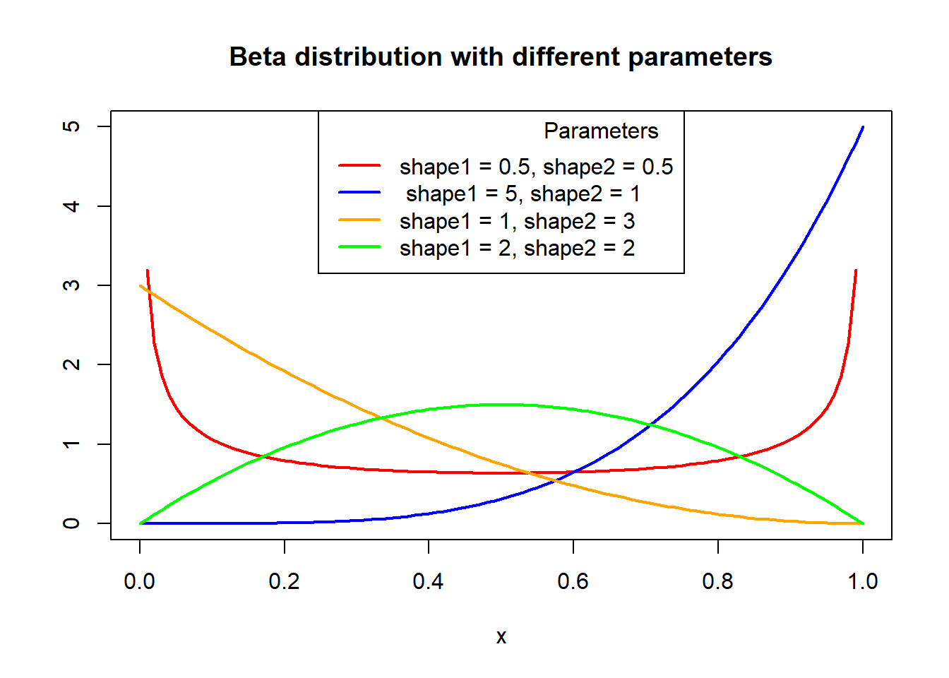
x <- seq(0, 1, 0.01)
plot(x, dbeta(x, shape1 = 0.5, shape2 = 0.5), type = "l", ylab = "", lwd = 2, col = "red", main = "Beta distribution with different parameters", ylim = c(0,5))

lines(x, dbeta(x, shape1 = 5, shape2 = 1), col = "blue", lty = 1, lwd = 2)

lines(x, dbeta(x, shape1 = 1, shape2 = 3), col = "orange", lty = 1, lwd = 2)


lines(x, dbeta(x, shape1 = 2, shape2 = 2), col = "green", lty = 1, lwd = 2)

# Adding a legend
legend("top", legend = c("shape1 = 0.5, shape2 = 0.5", " shape1 = 5, shape2 = 1", "shape1 = 1, shape2 = 3", "shape1 = 2, shape2 = 2"), col = c("red", "blue", "orange", "green"),
       title = "Parameters",
       title.adj = 0.9, lty = 1, lwd = 2)

Discrete Distributions

The Binomial Distribution

The Binomial Distribution is the distribution of success in \(n\) (fixed) number of trials involving binary(two outcomes) discrete random variables. Let \(X\) be number of success in

• fixed number of independent trails(\(n\)).
• Each trail has two possible outcomes: Success and failure
• Probability of success(\(p\)) is same in each trail.

\(X\) is said to follow binomial distribution \(X \sim bin(n,p)\), with parameters \(n\) and \(p\).

Mean and variance of binomial distribution:

• mean = \(n p\)

• Variance = \(n p (1-p)\)

The functions associated with the binomial distribution are used as follows:

dbinom(x= , size= , prob= )
pbinom(q= , size= , prob= , lower.tail= )
qbinom(p= , size= , prob= , lower.tail= )
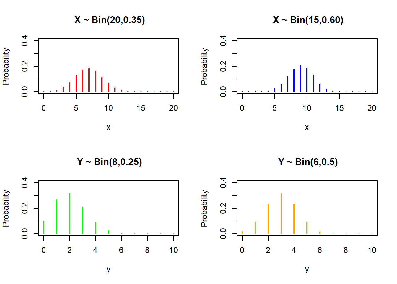
rbinom(n= , size= , prob= )

Graph of probability mass function for binomial distributions with different parameters;

See figure code

# Define discrete x-axis
x <- 0:20

par(mfrow = c(2, 2))

#Plot Binomial distribution
plot(x, dbinom(x, size = 20, prob = 0.35), type="h",
     ylim = c(0, 0.4), ylab = "Probability", main = " X ~ Bin(20,0.35)", lwd = 2, col = "red")

plot(x, dbinom(x, size = 15, prob = 0.60), type="h",
     ylim = c(0, 0.4), ylab = "Probability", main = " X ~ Bin(15,0.60)", lwd = 2, col = "blue")

y <- 0:10
plot(y, dbinom(y, size = 8, prob = 0.25), type="h",
     ylim = c(0, 0.4), ylab = "Probability", main = " Y ~ Bin(8,0.25)", lwd = 2, col = "green")

plot(y, dbinom(y, size = 6, prob = 0.50), type="h",
     ylim = c(0, 0.4), ylab = "Probability", main = " Y ~ Bin(6,0.5)", lwd = 2, col = "orange")

Example:

A fair coin is tossed 50 times, and we are interested in obtaining number of heads.

Let \(X\) be number of heads in 100 tosses, \(X \sim bin(100,0.5)\),

• Plot the probability mass function and compute probability that you will obtain exactly 25 heads?

answer

# Plot the probability density
xx <- 0:100
pxx<- dbinom(x=xx, size=100, prob=0.5)
plot( xx, pxx, type='h', col="red")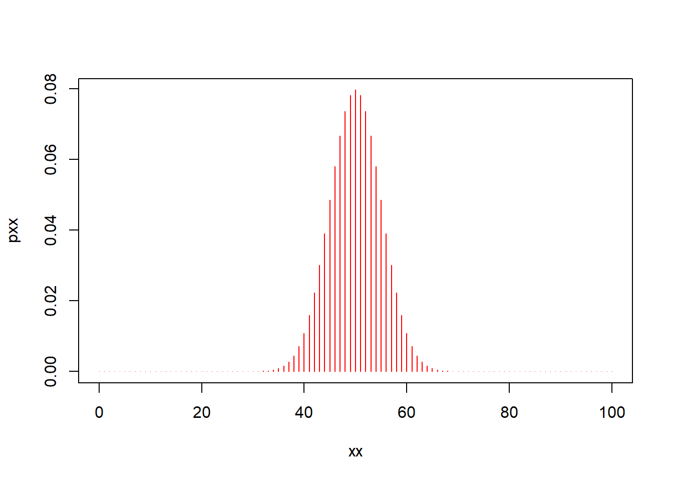

# Use dbinom to get the probability of exactly 25 heads
dbinom(x=25, size=100, prob=0.5)

## [1] 1.91314e-07

• Plot the probability distribution function and compute the probability of getting 20 or less heads?

answer

xx <- 0:100
dxx<- pbinom(q=xx, size=100, prob=0.5)
plot(xx, dxx, type='s', col="blue")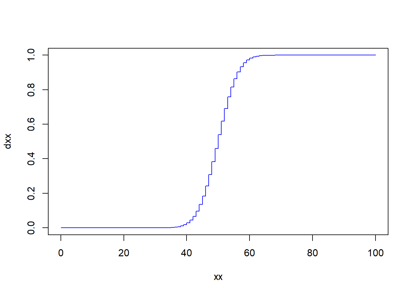

# Use pbinom to get the probability of 20 or less heads
pbinom(q=20, size=100, prob=0.5)

## [1] 5.579545e-10

• What is the probability that you will obtain more than 30 heads?

answer

The probability of getting greater than 30 heads is

\[P(X>30)=P(X \geq 31) = 1-P(x \leq 30)\] So we can use

1- pbinom(q = 30, size= 100, prob=0.5)

## [1] 0.9999607

# Alternatively we can specify that lower.tail =FALSE, if TRUE, we get P(X ≤ 30).
pbinom(q=30, size=100, prob= 0.5, lower.tail = FALSE)

## [1] 0.9999607

• What is the probability of getting between 15 and 20 heads?

answer

We want \(P(15 \leq X \leq 20)\), we can calculate this in following ways

pbinom(q=20, size=100, prob=0.5) - pbinom(q=15, size=100, prob=0.5) 

## [1] 5.577132e-10

#Equivalently 
diff(pbinom(q=c(15,20), size=100, prob = 0.5))

## [1] 5.577132e-10

• Find number of heads required so that 90% of the time, the number of head will be less than or equal to that number.

answer

qbinom(p=0.9, size=100, prob=0.5)

## [1] 56

• Generate 1000 samples from \(bin(100,0.5)\) and plot a histogram.

answer

rr <- rbinom(n=1000, size=100, prob=0.5)
hist(rr, plot=TRUE, breaks=20)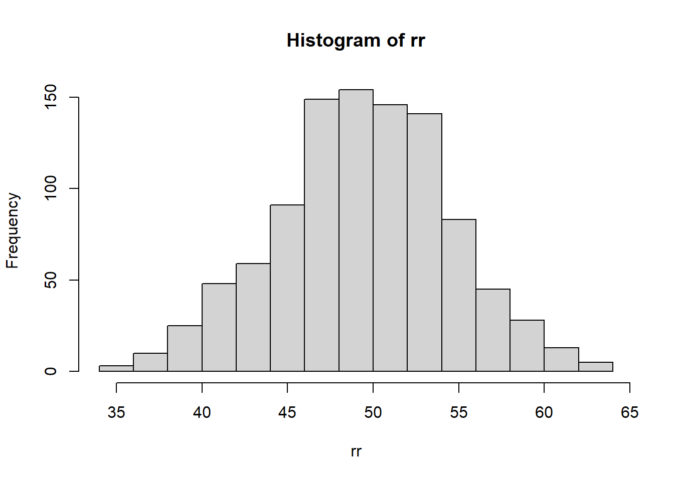

Poisson Distribution

The Poisson distribution is a discrete distribution used to model the number of events occurring within a fixed interval of time or space. It has one parameter \(\lambda\), which is the the average rate of occurrence.

For random variable \(X\) which follows Poisson distribution with mean number of events that occur at a given interval, \(\lambda\), we write \(X \sim Pois(\lambda)\).

Mean and variance of Poisson distribution:

• mean = \(\lambda\)

• Variance = $ $

The functions associated with the Poisson distribution are used as follows:

dpois(x= , lambda= )
ppois(q= , lambda= , lower.tail= )
qpois(p= , lambda= , lower.tail= )
rpois(n= , lambda= )

Graph of probability mass function of Poisson distributions with different parameters:

See figure code

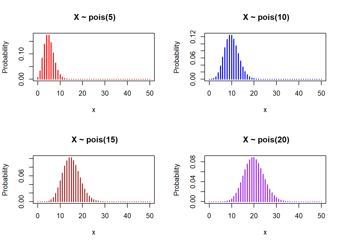
# Define discrete x-axis
x <- 0:50
par(mfrow = c(2, 2))

plot(x, dpois(x, 5), type="h" , ylab = "Probability", main = " X ~ pois(5)", lwd = 2, col = "red")

plot(x, dpois(x, 10), type="h", ylab = "Probability", main = " X ~ pois(10)", lwd = 2, col = "blue")

plot(x, dpois(x, 15), type="h", ylab = "Probability", main = " X ~ pois(15)", lwd = 2, col = "brown")

plot(x, dpois(x, 20), type="h", ylab = "Probability", main = " X ~ pois(20)", lwd = 2, col = "purple")

Geometric Distribution

The geometric distribution models the number of failures before a success is obtained in a sequence of independent Bernoulli trials, where each trial has the same probability of success. It has one parameter \(p\) which is the probability of success on each trial.

Let \(X\) be random variable which follows geometric distribution with probability of success at each trial equals \(p\), we write \(X \sim geom(p)\).

Mean and variance of geometric distribution:

• mean = \(\frac{1}{p}\)

• Variance = \(\frac{1-p}{p^2}\)

The functions associated with the geometric distribution are used as follows:

dgeom(x= , prob= )
pgeom(q= , prob= , lower.tail= )
qgeom(p= , prob= , lower.tail= )
rgeom(n= , prob= )

Graph of probability mass function of Poisson distributions with different parameters:

See figure code

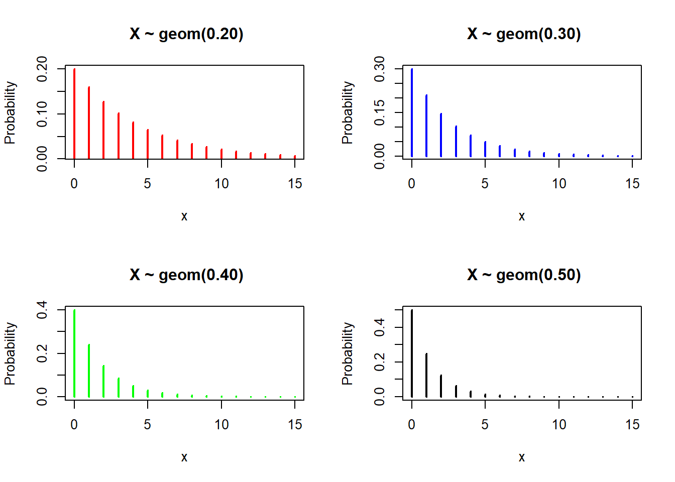
# Define discrete x-axis
x <- 0:15

par(mfrow = c(2, 2))


plot(x, dgeom(x,prob = 0.20), type="h",
     ylab = "Probability", main = " X ~ geom(0.20)", lwd = 2, col = "red")

plot(x, dgeom(x,prob = 0.30), type="h",
     ylab = "Probability", main = " X ~ geom(0.30)", lwd = 2, col = "blue")

plot(x, dgeom(x,prob = 0.40), type="h",
     ylab = "Probability", main = " X ~ geom(0.40)", lwd = 2, col = "green")

plot(x, dgeom(x,prob = 0.50), type="h",
     ylab = "Probability", main = " X ~ geom(0.50)", lwd = 2, col = "black")

Negative Binomial Distribution

The negative binomial distribution models the number of failures to observe a fixed number of successes in a sequence of Bernoulli trials with probability of success prob on each trial. It has two parameters, \(p\) which is the probability of success on each trial and \(r\) which is the number of success desired.

Let X be random variable which follows negative binomial distribution with probability of success at each trial equals \(p\), and we want \(r\) successes, then we write \(X \sim NB(r,p)\).

Mean and variance of negative binomial distribution:

• mean = \(\frac{r}{p}\)

• Variance = \(\frac{r(1-p)}{p^2}\)

The functions associated with the negative binomial distribution are used as follows:

dnbinom(x= , size= , prob= )
pnbinom(q= , size= , prob= , lower.tail = )
qnbinom(p= , size= , prob= , lower.tail = )
rnbinom(n= , size= , prob= )

Graph of probability mass function of negative binomial distribution with different parameters:

See figure code

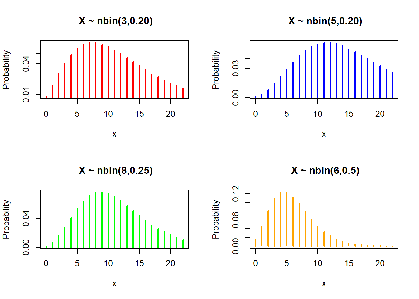
# Define discrete x-axis
x <- 0:22

par(mfrow = c(2, 2))

#Plot Binomial distribution
plot(x, dnbinom(x, size = 3, prob = 0.20), type="h",
     ylab = "Probability", main = " X ~ nbin(3,0.20)", lwd = 2, col = "red")

plot(x, dnbinom(x, size = 5, prob = 0.25), type="h",
      ylab = "Probability", main = " X ~ nbin(5,0.20)", lwd = 2, col = "blue")


plot(x, dnbinom(x, size = 6, prob = 0.35), type="h", 
     ylab = "Probability", main = " X ~ nbin(8,0.25)", lwd = 2, col = "green")

plot(x, dnbinom(x, size = 6, prob = 0.50), type="h",
     ylab = "Probability", main = " X ~ nbin(6,0.5)", lwd = 2, col = "orange")