Basic working with data
Reading data
When analysing data in R, the first step is typically you get your
data into an object called a data frame. One way to do this is manually
creating the data frame in R, but more often you will import the data
from an external file (typically some form of spreadsheet you might
normally open in excel). Various functions are available for importing
data into R, depending on the data file format. Commonly used functions
include read.csv() for CSV files, read.table()
for tab-delimited files, and readRDS() for R data
files.
Manually creating data
In R, we can create vectors of different data types using
c(). Lets create a numerical variable named
height, which is a vector representing height(cm) of 10
students as follows,
heights <- c(170, 165, 180, 160, 175, 168, 172, 178, 162, 170)
heights
## [1] 170 165 180 160 175 168 172 178 162 170Similarly we can create a categorical variable gender, which specifies the gender of each of the 10 individuals,
gender <- c("Male", "Female", "Male", "Female", "Male", "Male", "Female", "Male", "Female", "Male")

gender
## [1] "Male" "Female" "Male" "Female" "Male" "Male" "Female" "Male"
## [9] "Female" "Male"Data frames are used to store structured data with multiple
variables. We can create our own data using data.frame().
Here we created a new data frame named data, which contains
information about 10 individual’s gender and their height, using the
vectors we constructed above.
data <- data.frame(heights, gender)
data
## heights gender
## 1 170 Male
## 2 165 Female
## 3 180 Male
## 4 160 Female
## 5 175 Male
## 6 168 Male
## 7 172 Female
## 8 178 Male
## 9 162 Female
## 10 170 MaleReading Data Files with read.csv()
CSV files (‘csv’ stands for ‘comma separated values’) are common way
to store structured data in plain text format. Such files can be
imported into R using read.csv() as follows,
data <- read.csv("your_data.csv", header = TRUE)Here,
We need to replace
your_data.csvwith your actual file path and actual name of the data. You should put the data file in your project or your working directory, or a sub-directory of that.header=TRUE- when the first row of the csv file contains the variable names, otherwise useheader=FALSE.
For example: I want to import a CVS file saved as UNE_sleep.csv, which contains information about number of hours UNE students spent sleeping and name the dataset as une_sleep as follows,
une_sleep <- read.csv("Reading_data/Data sets/UNE_sleep.csv", header = TRUE)If your data were originally stored in an excel spreadsheet, you may have to save the sheet as a .csv file before you do this.
Reading Data Files with read.table()
The read.table() function is another of the commonly
used functions for reading files that contains tabular data into R. Lets
look at the syntax to import a .txt file using read
read.table()
data <- read.table("file name", header = FALSE, sep = "")By default, the function assumes that there is no header and the values are separated by white space. You can change them as per your file.
Example:
Here is a file called perch.txt in the Data Sets folder,
lets read it into R using read.table() function and name it
as data:
data <- read.table("Reading_data/Data sets/Perch.txt", header = TRUE)
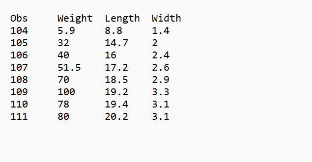
data## Obs Weight Length Width
## 1 104 5.9 8.8 1.4
## 2 105 32.0 14.7 2.0
## 3 106 40.0 16.0 2.4
## 4 107 51.5 17.2 2.6
## 5 108 70.0 18.5 2.9
## 6 109 100.0 19.2 3.3
## 7 110 78.0 19.4 3.1
## 8 111 80.0 20.2 3.1header =TRUE as the first row contains variable names.
Sep is not specified as it is separated by white space.
We can also import .txt files from internet using
read.table() function
data <- read.table("url", header = FALSE, sep = "")Using Built-in Datasets
There are many in-built datasets in R which can be used for
practicing and learning R. To read them in R, we can directly access
them using data(). For example, iris is an
in-built dataset which contains measurements of iris flowers. We can
read the data by
data("iris")The mtcars dataset provides information about various
car models, such as miles per gallon and horsepower, we can access it
by
data("mtcars")You can read the documentation about these datasets using,
? dataset_name,
?mtcarsData in excel spreadsheets
Typically if you only have a single dataset (e.g., a single sheet in
an excel file), the best practice would be to save it as a .csv file
before reading it into R. In some cases, you may have more complex data,
e.g., spread across multiple excel files or multiple sheets in in file.
In this case, you should consider reading data using a specialised
function from a package like read_xlsx() from the
readxl package. We will not detail this process here, as
most data you will encounter in coursework will be provided in .csv or
.txt format.
Exploring data
Once you have imported the data, we can explore the data using various functions in R. Some fundamental functions for exploring data in R are,
head()andtail(): These functions allow you to see the first few rows(head) and last few rows(tail) of the dataset.dim(): Allows you to check the number of rows and columns(dimension) of your dataset.names(): Allows to check the name of the variables of your dataset.str(): This function provides the summary of the structure of your dataset, showing the data types and first few values in each variable.summary(): This function provides summary statistics of numerical variables in your dataset.table(): It function is used to create frequency tables for categorical variables. It shows the counts of each category.mean(),median(),sd(),var(),IQR(): These functions can be used to generate numerical summaries like mean, median, standard deviation, variance, inter-quartile range respectively.
Iris examples
Let us apply the above function on the in-built dataset named ‘iris’,
- Lets load the dataset into R,
# Load the iris dataset
data(iris)- Lets check the first and last few rows of the dataset,
# View the first few rows of the dataset
head(iris)
## Sepal.Length Sepal.Width Petal.Length Petal.Width Species
## 1 5.1 3.5 1.4 0.2 setosa
## 2 4.9 3.0 1.4 0.2 setosa
## 3 4.7 3.2 1.3 0.2 setosa
## 4 4.6 3.1 1.5 0.2 setosa
## 5 5.0 3.6 1.4 0.2 setosa
## 6 5.4 3.9 1.7 0.4 setosa# View the last few rows of the dataset
tail(iris)## Sepal.Length Sepal.Width Petal.Length Petal.Width Species
## 145 6.7 3.3 5.7 2.5 virginica
## 146 6.7 3.0 5.2 2.3 virginica
## 147 6.3 2.5 5.0 1.9 virginica
## 148 6.5 3.0 5.2 2.0 virginica
## 149 6.2 3.4 5.4 2.3 virginica
## 150 5.9 3.0 5.1 1.8 virginica- Check th number of rows and columns(dimension) of your dataset,
dim(iris)## [1] 150 5There are 150 rows(observations) and 5 columns(variables).
- Check the name of the variables of your dataset,
names(iris)## [1] "Sepal.Length" "Sepal.Width" "Petal.Length" "Petal.Width" "Species"- Check the data types and first few values in each variable,
str(iris)## 'data.frame': 150 obs. of 5 variables:
## $ Sepal.Length: num 5.1 4.9 4.7 4.6 5 5.4 4.6 5 4.4 4.9 ...
## $ Sepal.Width : num 3.5 3 3.2 3.1 3.6 3.9 3.4 3.4 2.9 3.1 ...
## $ Petal.Length: num 1.4 1.4 1.3 1.5 1.4 1.7 1.4 1.5 1.4 1.5 ...
## $ Petal.Width : num 0.2 0.2 0.2 0.2 0.2 0.4 0.3 0.2 0.2 0.1 ...
## $ Species : Factor w/ 3 levels "setosa","versicolor",..: 1 1 1 1 1 1 1 1 1 1 ...We can see that first 4 variables are numerical but the \(5^{th}\) variables(Species) is categorical with 3 levels.
- Lets look at the summary statistics of the variables in your dataset,
summary(iris)## Sepal.Length Sepal.Width Petal.Length Petal.Width
## Min. :4.300 Min. :2.000 Min. :1.000 Min. :0.100
## 1st Qu.:5.100 1st Qu.:2.800 1st Qu.:1.600 1st Qu.:0.300
## Median :5.800 Median :3.000 Median :4.350 Median :1.300
## Mean :5.843 Mean :3.057 Mean :3.758 Mean :1.199
## 3rd Qu.:6.400 3rd Qu.:3.300 3rd Qu.:5.100 3rd Qu.:1.800
## Max. :7.900 Max. :4.400 Max. :6.900 Max. :2.500
## Species
## setosa :50
## versicolor:50
## virginica :50
##
##
## Notice that it gives numerical summary for the numerical variables and number of observations for categorical variable. There are 50 observations in each of the species.
Note: We can use $ to access single column in a data frame. If we want to generate the summary of Sepal.Width from the iris dataset, we can use
summary(iris$Sepal.Width)## Min. 1st Qu. Median Mean 3rd Qu. Max.
## 2.000 2.800 3.000 3.057 3.300 4.400- Lets look at the frequency for the categorical variable Species,
table(iris$Species)##
## setosa versicolor virginica
## 50 50 50- Lets calculate the mean, median, standard deviation, variance, inter-quartile range of the Petal.Length,
#mean of the Petal Length
mean(iris$Petal.Length)
## [1] 3.758#median of the Petal Length
median(iris$Petal.Length)## [1] 4.35#standard deviation of the Petal Length
sd(iris$Petal.Length)## [1] 1.765298#variance of the Petal Length
var(iris$Petal.Length)## [1] 3.116278#Inter-quartile range of the Petal Length
IQR(iris$Petal.Length)## [1] 3.5Numerical summaries by group
The tapply() function can be used to create summaries
based on categories as follows,
tapply(X, INDEX, FUN)Where
X: A numerical variable to apply a function toINDEX: A categorical variable to be grouped byFUN: The function to apply
Let us calculate the mean values of Petal.Length among different Species
## mean of petal length grouped by species

tapply(iris$Petal.Length, iris$Species, mean)
## setosa versicolor virginica
## 1.462 4.260 5.552Lets calculate the summaries of Sepal.Width among different Species
## summaries of sepal width grouped by species

tapply(iris$Sepal.Width, iris$Species, summary)
## $setosa
## Min. 1st Qu. Median Mean 3rd Qu. Max.
## 2.300 3.200 3.400 3.428 3.675 4.400
##
## $versicolor
## Min. 1st Qu. Median Mean 3rd Qu. Max.
## 2.000 2.525 2.800 2.770 3.000 3.400
##
## $virginica
## Min. 1st Qu. Median Mean 3rd Qu. Max.
## 2.200 2.800 3.000 2.974 3.175 3.800